


注意
前往結尾以下載完整的範例程式碼。
使用 Replay Buffers
作者: Vincent Moens
Replay buffers 是任何 RL 或控制演算法的核心。監督式學習方法的特點通常是一個訓練迴圈,其中資料是從靜態資料集中隨機提取,然後依序饋送到模型和損失函數。在 RL 中,情況通常略有不同:資料是使用模型收集的,然後暫時儲存在動態結構中(經驗回放緩衝區),該結構充當損失模組的資料集。
一如既往,使用緩衝區的環境會極大地影響其建構方式:有些人可能希望儲存軌跡,而另一些人則希望儲存單個轉換。在某些情況下,特定的抽樣策略可能更可取:某些項目的優先順序可能高於其他項目,或者以替換或不替換的方式進行抽樣可能很重要。計算因素也可能發揮作用,例如緩衝區的大小可能超過可用的 RAM 儲存空間。
由於這些原因,TorchRL 的 replay buffers 是完全可組合的:儘管它們帶有「電池已包含」的特性,只需最少的努力即可建構,但它們也支援許多自訂項目,例如儲存類型、抽樣策略或資料轉換。
在本教學中,您將學習
如何建構 Replay Buffer (RB) 並將其與任何資料類型一起使用;
如何自訂 緩衝區的儲存空間;
如何將 RBs 與 TensorDict 一起使用;
如何從 replay buffer 中抽樣或疊代,以及如何定義抽樣策略;
如何使用 優先排序的回放緩衝區;
如何 轉換 從緩衝區輸入和輸出的資料;
如何在緩衝區中儲存 軌跡。
基礎知識:建構 vanilla replay buffer
TorchRL 的 replay buffers 旨在優先考慮模組化、可組合性、效率和簡潔性。例如,建立基本 replay buffer 是一個簡單的過程,如下面的範例所示
import tempfile

from torchrl.data import ReplayBuffer

buffer = ReplayBuffer()
預設情況下,此 replay buffer 的大小為 1000。讓我們使用 extend() 方法來填充我們的緩衝區
print("length before adding elements:", len(buffer))

buffer.extend(range(2000))

print("length after adding elements:", len(buffer))
length before adding elements: 0
length after adding elements: 1000
我們使用了 extend() 方法,該方法旨在一次新增多個項目。如果傳遞給 extend 的物件有多個維度,則其第一個維度被認為是要在緩衝區中分割成獨立元素的維度。
這實際上意味著,當將多維張量或 tensordicts 新增到緩衝區時,緩衝區在計算其記憶體中保存的元素時,只會查看第一個維度。如果傳遞的物件不可疊代,則會引發異常。
若要一次新增一個項目,應改用 add() 方法。
自訂儲存空間
我們可以看到緩衝區已被限制為我們傳遞給它的前 1000 個元素。若要變更大小,我們需要自訂我們的儲存空間。
TorchRL 提供了三種類型的儲存空間:
ListStorage將元素獨立儲存在列表中。它支援任何資料類型,但這種靈活性會犧牲效率。LazyTensorStorage將張量資料結構連續儲存。 它可以自然地與TensorDict(或tensorclass) 物件搭配使用。 儲存空間在每個張量的基礎上是連續的,這表示採樣會比使用列表時更有效率,但隱含的限制是傳遞給它的任何資料都必須與用於實例化緩衝區的第一批資料具有相同的基本屬性(例如形狀和 dtype)。 傳遞不符合此需求的資料可能會引發例外,或導致一些未定義的行為。LazyMemmapStorage的工作方式與LazyTensorStorage相同,它是 lazy 的(也就是說,它期望第一批資料被實例化),並且它需要每個儲存的批次中的資料在形狀和 dtype 上匹配。 這種儲存空間的獨特之處在於它指向磁碟檔案(或使用檔案系統儲存),這意味著它可以支援非常大的資料集,同時仍然以連續的方式存取資料。
讓我們看看如何使用這些儲存空間
from torchrl.data import LazyMemmapStorage, LazyTensorStorage, ListStorage

# We define the maximum size of the buffer
size = 100
具有列表儲存緩衝區的緩衝區可以儲存任何類型的資料(但我們必須更改 collate_fn,因為預設值預期為數值資料)
buffer_list = ReplayBuffer(storage=ListStorage(size), collate_fn=lambda x: x)
buffer_list.extend(["a", 0, "b"])
print(buffer_list.sample(3))
['a', 'a', 0]
因為它是假設最少的,所以 ListStorage 是 TorchRL 中的預設儲存空間。
LazyTensorStorage 可以連續儲存資料。 在處理複雜但不變的中型資料結構時,這應該是首選選項
buffer_lazytensor = ReplayBuffer(storage=LazyTensorStorage(size))
讓我們建立一個大小為 ``torch.Size([3])` 的資料批次,其中儲存了 2 個張量
import torch
from tensordict import TensorDict

data = TensorDict(
    {
        "a": torch.arange(12).view(3, 4),
        ("b", "c"): torch.arange(15).view(3, 5),
    },
    batch_size=[3],
)
print(data)
TensorDict(
    fields={
        a: Tensor(shape=torch.Size([3, 4]), device=cpu, dtype=torch.int64, is_shared=False),
        b: TensorDict(
            fields={
                c: Tensor(shape=torch.Size([3, 5]), device=cpu, dtype=torch.int64, is_shared=False)},
            batch_size=torch.Size([3]),
            device=None,
            is_shared=False)},
    batch_size=torch.Size([3]),
    device=None,
    is_shared=False)
第一次呼叫 extend() 將會實例化儲存空間。 資料的第一個維度會被解綁到單獨的資料點中
buffer_lazytensor.extend(data)
print(f"The buffer has {len(buffer_lazytensor)} elements")
The buffer has 3 elements
讓我們從緩衝區中取樣,並列印資料
sample = buffer_lazytensor.sample(5)
print("samples", sample["a"], sample["b", "c"])
samples tensor([[0, 1, 2, 3],
        [0, 1, 2, 3],
        [4, 5, 6, 7],
        [0, 1, 2, 3],
        [0, 1, 2, 3]]) tensor([[0, 1, 2, 3, 4],
        [0, 1, 2, 3, 4],
        [5, 6, 7, 8, 9],
        [0, 1, 2, 3, 4],
        [0, 1, 2, 3, 4]])
LazyMemmapStorage 的建立方式相同
buffer_lazymemmap = ReplayBuffer(storage=LazyMemmapStorage(size))
buffer_lazymemmap.extend(data)
print(f"The buffer has {len(buffer_lazymemmap)} elements")
sample = buffer_lazytensor.sample(5)
print("samples: a=", sample["a"], "\n('b', 'c'):", sample["b", "c"])
The buffer has 3 elements
samples: a= tensor([[ 0,  1,  2,  3],
        [ 0,  1,  2,  3],
        [ 0,  1,  2,  3],
        [ 8,  9, 10, 11],
        [ 8,  9, 10, 11]])
('b', 'c'): tensor([[ 0,  1,  2,  3,  4],
        [ 0,  1,  2,  3,  4],
        [ 0,  1,  2,  3,  4],
        [10, 11, 12, 13, 14],
        [10, 11, 12, 13, 14]])
我們也可以自訂磁碟上的儲存位置
tempdir = tempfile.TemporaryDirectory()
buffer_lazymemmap = ReplayBuffer(storage=LazyMemmapStorage(size, scratch_dir=tempdir))
buffer_lazymemmap.extend(data)
print(f"The buffer has {len(buffer_lazymemmap)} elements")
print("the 'a' tensor is stored in", buffer_lazymemmap._storage._storage["a"].filename)
print(
    "the ('b', 'c') tensor is stored in",
    buffer_lazymemmap._storage._storage["b", "c"].filename,
)
The buffer has 3 elements
the 'a' tensor is stored in /pytorch/rl/docs/source/reference/generated/tutorials/<TemporaryDirectory '/tmp/tmpzxmvjdim'>/a.memmap
the ('b', 'c') tensor is stored in /pytorch/rl/docs/source/reference/generated/tutorials/<TemporaryDirectory '/tmp/tmpzxmvjdim'>/b/c.memmap
與 TensorDict 整合
張量位置遵循與包含它們的 TensorDict 相同的結構:這使得在訓練期間可以輕鬆儲存和載入緩衝區。
若要充分利用 TensorDict 作為資料載體,可以使用 TensorDictReplayBuffer 類別。 它的主要優點之一是能夠處理取樣資料的組織,以及可能需要的任何額外資訊(例如取樣索引)。
它可以像標準 ReplayBuffer 一樣建構,並且通常可以互換使用。
from torchrl.data import TensorDictReplayBuffer

tempdir = tempfile.TemporaryDirectory()
buffer_lazymemmap = TensorDictReplayBuffer(
    storage=LazyMemmapStorage(size, scratch_dir=tempdir), batch_size=12
)
buffer_lazymemmap.extend(data)
print(f"The buffer has {len(buffer_lazymemmap)} elements")
sample = buffer_lazymemmap.sample()
print("sample:", sample)
The buffer has 3 elements
sample: TensorDict(
    fields={
        a: Tensor(shape=torch.Size([12, 4]), device=cpu, dtype=torch.int64, is_shared=False),
        b: TensorDict(
            fields={
                c: Tensor(shape=torch.Size([12, 5]), device=cpu, dtype=torch.int64, is_shared=False)},
            batch_size=torch.Size([12]),
            device=cpu,
            is_shared=False),
        index: Tensor(shape=torch.Size([12]), device=cpu, dtype=torch.int64, is_shared=False)},
    batch_size=torch.Size([12]),
    device=cpu,
    is_shared=False)
我們的樣本現在有一個額外的 "index" 鍵,指示取樣了哪些索引。 讓我們看看這些索引
print(sample["index"])
tensor([2, 1, 2, 1, 0, 0, 1, 2, 0, 0, 0, 2])
與 tensorclass 整合
ReplayBuffer 類別和相關的子類別也可以與 tensorclass 類別原生運作,後者可以方便地用於以更明確的方式編碼資料集
from tensordict import tensorclass


@tensorclass
class MyData:
    images: torch.Tensor
    labels: torch.Tensor


data = MyData(
    images=torch.randint(
        255,
        (10, 64, 64, 3),
    ),
    labels=torch.randint(100, (10,)),
    batch_size=[10],
)

tempdir = tempfile.TemporaryDirectory()
buffer_lazymemmap = ReplayBuffer(
    storage=LazyMemmapStorage(size, scratch_dir=tempdir), batch_size=12
)
buffer_lazymemmap.extend(data)
print(f"The buffer has {len(buffer_lazymemmap)} elements")
sample = buffer_lazymemmap.sample()
print("sample:", sample)
The buffer has 10 elements
sample: MyData(
    images=Tensor(shape=torch.Size([12, 64, 64, 3]), device=cpu, dtype=torch.int64, is_shared=False),
    labels=Tensor(shape=torch.Size([12]), device=cpu, dtype=torch.int64, is_shared=False),
    batch_size=torch.Size([12]),
    device=cpu,
    is_shared=False)
如預期的,資料具有正確的類別和形狀!
與其他張量結構 (PyTrees) 整合
TorchRL 的重播緩衝區也可以與任何 pytree 資料結構一起運作。 PyTree 是一種由 dict、list 和/或 tuple 組成的任意深度巢狀結構,其中葉子是張量。 這意味著可以將任何此類樹狀結構儲存在連續記憶體中! 可以使用各種儲存空間: TensorStorage、 LazyMemmapStorage 或 LazyTensorStorage 都接受這種資料。
以下是此功能的外觀的簡要示範
from torch.utils._pytree import tree_map
讓我們在磁碟上建構我們的重播緩衝區
rb = ReplayBuffer(storage=LazyMemmapStorage(size))
data = {
    "a": torch.randn(3),
    "b": {"c": (torch.zeros(2), [torch.ones(1)])},
    30: -torch.ones(()),  # non-string keys also work
}
rb.add(data)

# The sample has a similar structure to the data (with a leading dimension of 10 for each tensor)
sample = rb.sample(10)
使用 pytrees,任何可呼叫的物件都可以用作轉換
def transform(x):
    # Zeros all the data in the pytree
    return tree_map(lambda y: y * 0, x)


rb.append_transform(transform)
sample = rb.sample(batch_size=12)
讓我們檢查一下我們的轉換是否完成了它的工作
def assert0(x):
    assert (x == 0).all()


tree_map(assert0, sample)
{'a': None, 'b': {'c': (None, [None])}, 30: None}
取樣和迭代緩衝區
重播緩衝區支援多種取樣策略
如果批次大小是固定的並且可以在建構時定義,則可以將其作為關鍵字引數傳遞給緩衝區。
使用固定批次大小,可以迭代重播緩衝區以收集樣本。
如果批次大小是動態的,則可以將其傳遞給
sample方法。
可以使用多執行緒進行取樣,但這與最後一個選項不相容(因為它要求緩衝區預先知道下一個批次的大小)。
讓我們看幾個範例
固定批次大小
如果在建構期間傳遞了批次大小,則在取樣時應省略它
data = MyData(
    images=torch.randint(
        255,
        (200, 64, 64, 3),
    ),
    labels=torch.randint(100, (200,)),
    batch_size=[200],
)

buffer_lazymemmap = ReplayBuffer(storage=LazyMemmapStorage(size), batch_size=128)
buffer_lazymemmap.extend(data)
buffer_lazymemmap.sample()
MyData(
    images=Tensor(shape=torch.Size([128, 64, 64, 3]), device=cpu, dtype=torch.int64, is_shared=False),
    labels=Tensor(shape=torch.Size([128]), device=cpu, dtype=torch.int64, is_shared=False),
    batch_size=torch.Size([128]),
    device=cpu,
    is_shared=False)
此資料批次具有我們希望它具有的大小 (128)。
若要啟用多執行緒取樣,只需在建構期間將正整數傳遞給 prefetch 關鍵字引數。 每當取樣耗時(例如,使用優先取樣器時),這應該會大大加快取樣速度
buffer_lazymemmap = ReplayBuffer(
    storage=LazyMemmapStorage(size), batch_size=128, prefetch=10
)  # creates a queue of 10 elements to be prefetched in the background
buffer_lazymemmap.extend(data)
print(buffer_lazymemmap.sample())
MyData(
    images=Tensor(shape=torch.Size([128, 64, 64, 3]), device=cpu, dtype=torch.int64, is_shared=False),
    labels=Tensor(shape=torch.Size([128]), device=cpu, dtype=torch.int64, is_shared=False),
    batch_size=torch.Size([128]),
    device=cpu,
    is_shared=False)
使用固定批次大小迭代緩衝區
我們也可以像使用常規資料載入器一樣迭代緩衝區,只要預先定義了批次大小
for i, data in enumerate(buffer_lazymemmap):
    if i == 3:
        print(data)
        break
MyData(
    images=Tensor(shape=torch.Size([128, 64, 64, 3]), device=cpu, dtype=torch.int64, is_shared=False),
    labels=Tensor(shape=torch.Size([128]), device=cpu, dtype=torch.int64, is_shared=False),
    batch_size=torch.Size([128]),
    device=cpu,
    is_shared=False)
由於我們的抽樣技術是完全隨機的,且不阻止重複取樣,因此迭代器是無限的。然而,我們可以改用 SamplerWithoutReplacement,它會將我們的緩衝區轉換為有限的迭代器。
from torchrl.data.replay_buffers.samplers import SamplerWithoutReplacement

buffer_lazymemmap = ReplayBuffer(
    storage=LazyMemmapStorage(size), batch_size=32, sampler=SamplerWithoutReplacement()
)
我們創建足夠大的資料,以便取得幾個樣本。
data = TensorDict(
    {
        "a": torch.arange(64).view(16, 4),
        ("b", "c"): torch.arange(128).view(16, 8),
    },
    batch_size=[16],
)

buffer_lazymemmap.extend(data)
for _i, _ in enumerate(buffer_lazymemmap):
    continue
print(f"A total of {_i+1} batches have been collected")
A total of 1 batches have been collected
動態批次大小
與我們之前看到的相反,可以省略 batch_size 關鍵字引數,並直接傳遞給 sample 方法。
buffer_lazymemmap = ReplayBuffer(
    storage=LazyMemmapStorage(size), sampler=SamplerWithoutReplacement()
)
buffer_lazymemmap.extend(data)
print("sampling 3 elements:", buffer_lazymemmap.sample(3))
print("sampling 5 elements:", buffer_lazymemmap.sample(5))
sampling 3 elements: TensorDict(
    fields={
        a: Tensor(shape=torch.Size([3, 4]), device=cpu, dtype=torch.int64, is_shared=False),
        b: TensorDict(
            fields={
                c: Tensor(shape=torch.Size([3, 8]), device=cpu, dtype=torch.int64, is_shared=False)},
            batch_size=torch.Size([3]),
            device=cpu,
            is_shared=False)},
    batch_size=torch.Size([3]),
    device=cpu,
    is_shared=False)
sampling 5 elements: TensorDict(
    fields={
        a: Tensor(shape=torch.Size([5, 4]), device=cpu, dtype=torch.int64, is_shared=False),
        b: TensorDict(
            fields={
                c: Tensor(shape=torch.Size([5, 8]), device=cpu, dtype=torch.int64, is_shared=False)},
            batch_size=torch.Size([5]),
            device=cpu,
            is_shared=False)},
    batch_size=torch.Size([5]),
    device=cpu,
    is_shared=False)
優先權重播緩衝區
TorchRL 也提供了一個 優先權重播緩衝區 的介面。這個緩衝區類別會根據透過資料傳遞的優先權訊號來抽樣資料。
雖然這個工具與非 TensorDict 資料相容,但我們鼓勵使用 TensorDict,因為它能輕鬆地從緩衝區中攜帶元資料進出。
讓我們首先看看如何在一般情況下建立優先權重播緩衝區。 \(\alpha\) 和 \(\beta\) 超參數必須手動設定。
from torchrl.data.replay_buffers.samplers import PrioritizedSampler

size = 100

rb = ReplayBuffer(
    storage=ListStorage(size),
    sampler=PrioritizedSampler(max_capacity=size, alpha=0.8, beta=1.1),
    collate_fn=lambda x: x,
)
擴充重播緩衝區會傳回項目索引,我們稍後需要這些索引來更新優先權。
indices = rb.extend([1, "foo", None])
抽樣器期望每個元素都有一個優先權。新增到緩衝區時,優先權會設定為預設值 1。一旦計算出優先權(通常是透過損失),就必須在緩衝區中更新它。
這是透過 update_priority() 方法完成的,該方法需要索引以及優先權。我們為資料集中的第二個樣本分配一個人為的高優先權,以觀察其對抽樣的影響。
rb.update_priority(index=indices, priority=torch.tensor([0, 1_000, 0.1]))
我們觀察到從緩衝區抽樣主要傳回第二個樣本("foo")。
sample, info = rb.sample(10, return_info=True)
print(sample)
['foo', 'foo', 'foo', 'foo', 'foo', 'foo', 'foo', 'foo', 'foo', 'foo']
資訊包含項目的相對權重以及索引。
print(info)
{'_weight': tensor([2.0893e-10, 2.0893e-10, 2.0893e-10, 2.0893e-10, 2.0893e-10, 2.0893e-10,
        2.0893e-10, 2.0893e-10, 2.0893e-10, 2.0893e-10]), 'index': tensor([1, 1, 1, 1, 1, 1, 1, 1, 1, 1])}
我們看到,與常規緩衝區相比,使用優先權重播緩衝區需要在訓練迴圈中執行一系列額外的步驟。
收集資料並擴充緩衝區後,必須更新項目的優先權;
在計算損失並從中獲得「優先權訊號」後,我們必須再次更新緩衝區中項目的優先權。這需要我們追蹤索引。
這會大幅降低緩衝區的重複使用性:如果有人要編寫一個訓練腳本,其中可以建立優先權重播緩衝區和常規緩衝區,則她必須新增大量的控制流程,以確保在適當的位置呼叫適當的方法,前提是正在使用優先權重播緩衝區。
讓我們看看如何使用 TensorDict 來改善這一點。我們看到 TensorDictReplayBuffer 傳回的資料會以其相對儲存索引擴增。我們沒有提到的一個特性是,如果擴充期間存在優先權訊號,這個類別也會確保自動將優先權訊號剖析到優先權抽樣器。
這些功能的組合簡化了許多事情:- 擴充緩衝區時,優先權訊號將自動
在存在的情況下進行剖析,並且將準確地分配優先權;
索引將儲存在抽樣的 tensordict 中,使其易於在損失計算後更新優先權。
在計算損失時,優先權訊號將註冊到傳遞給損失模組的 tensordict 中,從而可以毫不費力地更新權重。
>>> data = replay_buffer.sample()
>>> loss_val = loss_module(data)
>>> replay_buffer.update_tensordict_priority(data)
以下程式碼說明了這些概念。我們建立一個具有優先權抽樣器的重播緩衝區,並在建構函式中指示應提取優先權訊號的條目。
rb = TensorDictReplayBuffer(
    storage=ListStorage(size),
    sampler=PrioritizedSampler(size, alpha=0.8, beta=1.1),
    priority_key="td_error",
    batch_size=1024,
)
讓我們選擇一個與儲存索引成比例的優先權訊號。
data["td_error"] = torch.arange(data.numel())

rb.extend(data)

sample = rb.sample()
較高的索引應更頻繁地出現。
from matplotlib import pyplot as plt

plt.hist(sample["index"].numpy())
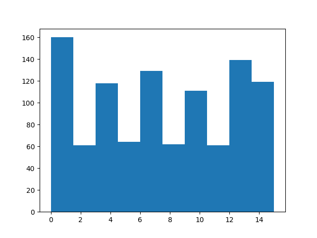
(array([160., 61., 118., 64., 129., 62., 111., 61., 139., 119.]), array([ 0. , 1.5, 3. , 4.5, 6. , 7.5, 9. , 10.5, 12. , 13.5, 15. ]), <BarContainer object of 10 artists>)
一旦我們處理完樣本,我們就使用 torchrl.data.TensorDictReplayBuffer.update_tensordict_priority() 方法更新優先權鍵。為了展示這是如何運作的,讓我們恢復抽樣項目的優先權。
sample = rb.sample()
sample["td_error"] = data.numel() - sample["index"]
rb.update_tensordict_priority(sample)
現在,較高的索引應較少出現。
sample = rb.sample()
from matplotlib import pyplot as plt

plt.hist(sample["index"].numpy())
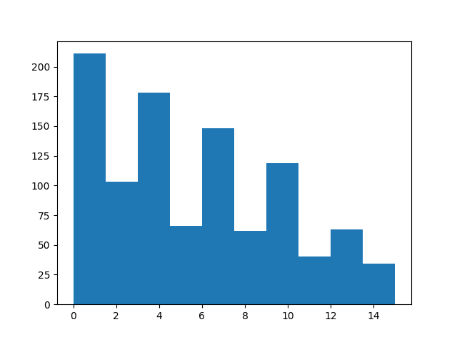
(array([211., 103., 178., 66., 148., 62., 119., 40., 63., 34.]), array([ 0. , 1.5, 3. , 4.5, 6. , 7.5, 9. , 10.5, 12. , 13.5, 15. ]), <BarContainer object of 10 artists>)
使用轉換
儲存在重播緩衝區中的資料可能尚未準備好呈現給損失模組。在某些情況下,收集器產生的資料可能太重,無法按原樣儲存。這方面的範例包括將影像從 uint8 轉換為浮點張量,或在使用決策轉換器時串聯連續的幀。
只需將適當的轉換附加到緩衝區,即可在緩衝區內外處理資料。以下是一些範例:
儲存原始影像
uint8 類型的張量比我們通常饋送到模型的浮點張量在記憶體上的花費相對較少。因此,儲存原始影像可能很有用。以下腳本示範瞭如何建立一個僅傳回原始影像的收集器,但使用轉換後的影像進行推論,以及如何在重播緩衝區中回收這些轉換。
from torchrl.collectors import SyncDataCollector
from torchrl.envs.libs.gym import GymEnv
from torchrl.envs.transforms import (
    Compose,
    GrayScale,
    Resize,
    ToTensorImage,
    TransformedEnv,
)
from torchrl.envs.utils import RandomPolicy

env = TransformedEnv(
    GymEnv("CartPole-v1", from_pixels=True),
    Compose(
        ToTensorImage(in_keys=["pixels"], out_keys=["pixels_trsf"]),
        Resize(in_keys=["pixels_trsf"], w=64, h=64),
        GrayScale(in_keys=["pixels_trsf"]),
    ),
)
讓我們看看一個 rollout。
print(env.rollout(3))
TensorDict(
    fields={
        action: Tensor(shape=torch.Size([3, 2]), device=cpu, dtype=torch.int64, is_shared=False),
        done: Tensor(shape=torch.Size([3, 1]), device=cpu, dtype=torch.bool, is_shared=False),
        next: TensorDict(
            fields={
                done: Tensor(shape=torch.Size([3, 1]), device=cpu, dtype=torch.bool, is_shared=False),
                pixels: Tensor(shape=torch.Size([3, 400, 600, 3]), device=cpu, dtype=torch.uint8, is_shared=False),
                pixels_trsf: Tensor(shape=torch.Size([3, 1, 64, 64]), device=cpu, dtype=torch.float32, is_shared=False),
                reward: Tensor(shape=torch.Size([3, 1]), device=cpu, dtype=torch.float32, is_shared=False),
                terminated: Tensor(shape=torch.Size([3, 1]), device=cpu, dtype=torch.bool, is_shared=False),
                truncated: Tensor(shape=torch.Size([3, 1]), device=cpu, dtype=torch.bool, is_shared=False)},
            batch_size=torch.Size([3]),
            device=None,
            is_shared=False),
        pixels: Tensor(shape=torch.Size([3, 400, 600, 3]), device=cpu, dtype=torch.uint8, is_shared=False),
        pixels_trsf: Tensor(shape=torch.Size([3, 1, 64, 64]), device=cpu, dtype=torch.float32, is_shared=False),
        terminated: Tensor(shape=torch.Size([3, 1]), device=cpu, dtype=torch.bool, is_shared=False),
        truncated: Tensor(shape=torch.Size([3, 1]), device=cpu, dtype=torch.bool, is_shared=False)},
    batch_size=torch.Size([3]),
    device=None,
    is_shared=False)
我們剛剛建立了一個產生像素的環境。這些影像是經過處理的,以便饋送到策略。我們想要儲存原始影像,而不是其轉換。為此,我們將轉換附加到收集器,以選擇我們想要看到的鍵。
from torchrl.envs.transforms import ExcludeTransform

collector = SyncDataCollector(
    env,
    RandomPolicy(env.action_spec),
    frames_per_batch=10,
    total_frames=1000,
    postproc=ExcludeTransform("pixels_trsf", ("next", "pixels_trsf"), "collector"),
)
讓我們看看一批資料,並控制 "pixels_trsf" 鍵是否已被丟棄。
for data in collector:
    print(data)
    break
TensorDict(
    fields={
        action: Tensor(shape=torch.Size([10, 2]), device=cpu, dtype=torch.int64, is_shared=False),
        done: Tensor(shape=torch.Size([10, 1]), device=cpu, dtype=torch.bool, is_shared=False),
        next: TensorDict(
            fields={
                done: Tensor(shape=torch.Size([10, 1]), device=cpu, dtype=torch.bool, is_shared=False),
                pixels: Tensor(shape=torch.Size([10, 400, 600, 3]), device=cpu, dtype=torch.uint8, is_shared=False),
                reward: Tensor(shape=torch.Size([10, 1]), device=cpu, dtype=torch.float32, is_shared=False),
                terminated: Tensor(shape=torch.Size([10, 1]), device=cpu, dtype=torch.bool, is_shared=False),
                truncated: Tensor(shape=torch.Size([10, 1]), device=cpu, dtype=torch.bool, is_shared=False)},
            batch_size=torch.Size([10]),
            device=None,
            is_shared=False),
        pixels: Tensor(shape=torch.Size([10, 400, 600, 3]), device=cpu, dtype=torch.uint8, is_shared=False),
        terminated: Tensor(shape=torch.Size([10, 1]), device=cpu, dtype=torch.bool, is_shared=False),
        truncated: Tensor(shape=torch.Size([10, 1]), device=cpu, dtype=torch.bool, is_shared=False)},
    batch_size=torch.Size([10]),
    device=None,
    is_shared=False)
我們建立一個與環境具有相同轉換的重播緩衝區。但是,有一個需要解決的細節:未使用環境的轉換不會注意到資料結構。將轉換附加到環境時,"next" 巢狀 tensordict 中的資料會首先進行轉換,然後在 rollout 執行期間複製到根目錄。處理靜態資料時,情況並非如此。儘管如此,我們的資料帶有一個巢狀的「next」tensordict,如果我們沒有明確指示它注意它,我們的轉換將忽略它。我們手動將這些鍵新增到轉換。
t = Compose(
    ToTensorImage(
        in_keys=["pixels", ("next", "pixels")],
        out_keys=["pixels_trsf", ("next", "pixels_trsf")],
    ),
    Resize(in_keys=["pixels_trsf", ("next", "pixels_trsf")], w=64, h=64),
    GrayScale(in_keys=["pixels_trsf", ("next", "pixels_trsf")]),
)
rb = TensorDictReplayBuffer(storage=LazyMemmapStorage(1000), transform=t, batch_size=16)
rb.extend(data)
tensor([0, 1, 2, 3, 4, 5, 6, 7, 8, 9])
我們可以檢查 sample 方法是否看到轉換後的影像重新出現。
print(rb.sample())
TensorDict(
    fields={
        action: Tensor(shape=torch.Size([16, 2]), device=cpu, dtype=torch.int64, is_shared=False),
        done: Tensor(shape=torch.Size([16, 1]), device=cpu, dtype=torch.bool, is_shared=False),
        index: Tensor(shape=torch.Size([16]), device=cpu, dtype=torch.int64, is_shared=False),
        next: TensorDict(
            fields={
                done: Tensor(shape=torch.Size([16, 1]), device=cpu, dtype=torch.bool, is_shared=False),
                pixels: Tensor(shape=torch.Size([16, 400, 600, 3]), device=cpu, dtype=torch.uint8, is_shared=False),
                pixels_trsf: Tensor(shape=torch.Size([16, 1, 64, 64]), device=cpu, dtype=torch.float32, is_shared=False),
                reward: Tensor(shape=torch.Size([16, 1]), device=cpu, dtype=torch.float32, is_shared=False),
                terminated: Tensor(shape=torch.Size([16, 1]), device=cpu, dtype=torch.bool, is_shared=False),
                truncated: Tensor(shape=torch.Size([16, 1]), device=cpu, dtype=torch.bool, is_shared=False)},
            batch_size=torch.Size([16]),
            device=cpu,
            is_shared=False),
        pixels: Tensor(shape=torch.Size([16, 400, 600, 3]), device=cpu, dtype=torch.uint8, is_shared=False),
        pixels_trsf: Tensor(shape=torch.Size([16, 1, 64, 64]), device=cpu, dtype=torch.float32, is_shared=False),
        terminated: Tensor(shape=torch.Size([16, 1]), device=cpu, dtype=torch.bool, is_shared=False),
        truncated: Tensor(shape=torch.Size([16, 1]), device=cpu, dtype=torch.bool, is_shared=False)},
    batch_size=torch.Size([16]),
    device=cpu,
    is_shared=False)
更複雜的範例:使用 CatFrames
CatFrames 轉換會將觀測值隨著時間展開,建立一個 n-back 的過去事件記憶,讓模型可以將過去的事件納入考量(在 POMDPs 的情況下,或是使用遞迴策略,例如 Decision Transformers)。儲存這些串聯的幀可能會消耗相當多的記憶體。當 n-back 視窗需要在訓練和推論期間有所不同(通常是更長)時,也可能產生問題。我們透過在兩個階段分別執行 CatFrames 轉換來解決這個問題。
from torchrl.envs import CatFrames, UnsqueezeTransform
我們為返回基於像素的觀測值的環境建立一個標準的轉換列表。
env = TransformedEnv(
    GymEnv("CartPole-v1", from_pixels=True),
    Compose(
        ToTensorImage(in_keys=["pixels"], out_keys=["pixels_trsf"]),
        Resize(in_keys=["pixels_trsf"], w=64, h=64),
        GrayScale(in_keys=["pixels_trsf"]),
        UnsqueezeTransform(-4, in_keys=["pixels_trsf"]),
        CatFrames(dim=-4, N=4, in_keys=["pixels_trsf"]),
    ),
)
collector = SyncDataCollector(
    env,
    RandomPolicy(env.action_spec),
    frames_per_batch=10,
    total_frames=1000,
)
for data in collector:
    print(data)
    break
TensorDict(
    fields={
        action: Tensor(shape=torch.Size([10, 2]), device=cpu, dtype=torch.int64, is_shared=False),
        collector: TensorDict(
            fields={
                traj_ids: Tensor(shape=torch.Size([10]), device=cpu, dtype=torch.int64, is_shared=False)},
            batch_size=torch.Size([10]),
            device=None,
            is_shared=False),
        done: Tensor(shape=torch.Size([10, 1]), device=cpu, dtype=torch.bool, is_shared=False),
        next: TensorDict(
            fields={
                done: Tensor(shape=torch.Size([10, 1]), device=cpu, dtype=torch.bool, is_shared=False),
                pixels: Tensor(shape=torch.Size([10, 400, 600, 3]), device=cpu, dtype=torch.uint8, is_shared=False),
                pixels_trsf: Tensor(shape=torch.Size([10, 4, 1, 64, 64]), device=cpu, dtype=torch.float32, is_shared=False),
                reward: Tensor(shape=torch.Size([10, 1]), device=cpu, dtype=torch.float32, is_shared=False),
                terminated: Tensor(shape=torch.Size([10, 1]), device=cpu, dtype=torch.bool, is_shared=False),
                truncated: Tensor(shape=torch.Size([10, 1]), device=cpu, dtype=torch.bool, is_shared=False)},
            batch_size=torch.Size([10]),
            device=None,
            is_shared=False),
        pixels: Tensor(shape=torch.Size([10, 400, 600, 3]), device=cpu, dtype=torch.uint8, is_shared=False),
        pixels_trsf: Tensor(shape=torch.Size([10, 4, 1, 64, 64]), device=cpu, dtype=torch.float32, is_shared=False),
        terminated: Tensor(shape=torch.Size([10, 1]), device=cpu, dtype=torch.bool, is_shared=False),
        truncated: Tensor(shape=torch.Size([10, 1]), device=cpu, dtype=torch.bool, is_shared=False)},
    batch_size=torch.Size([10]),
    device=None,
    is_shared=False)
緩衝區轉換看起來很像環境轉換,但帶有額外的 ("next", ...) 鍵,就像之前一樣。
t = Compose(
    ToTensorImage(
        in_keys=["pixels", ("next", "pixels")],
        out_keys=["pixels_trsf", ("next", "pixels_trsf")],
    ),
    Resize(in_keys=["pixels_trsf", ("next", "pixels_trsf")], w=64, h=64),
    GrayScale(in_keys=["pixels_trsf", ("next", "pixels_trsf")]),
    UnsqueezeTransform(-4, in_keys=["pixels_trsf", ("next", "pixels_trsf")]),
    CatFrames(dim=-4, N=4, in_keys=["pixels_trsf", ("next", "pixels_trsf")]),
)
rb = TensorDictReplayBuffer(storage=LazyMemmapStorage(size), transform=t, batch_size=16)
data_exclude = data.exclude("pixels_trsf", ("next", "pixels_trsf"))
rb.add(data_exclude)
0
讓我們從緩衝區中抽樣一個批次。轉換後的像素鍵的形狀應該在從結尾開始的第四個維度上具有長度為 4。
s = rb.sample(1)  # the buffer has only one element
print(s)
TensorDict(
    fields={
        action: Tensor(shape=torch.Size([1, 10, 2]), device=cpu, dtype=torch.int64, is_shared=False),
        collector: TensorDict(
            fields={
                traj_ids: Tensor(shape=torch.Size([1, 10]), device=cpu, dtype=torch.int64, is_shared=False)},
            batch_size=torch.Size([1, 10]),
            device=cpu,
            is_shared=False),
        done: Tensor(shape=torch.Size([1, 10, 1]), device=cpu, dtype=torch.bool, is_shared=False),
        index: Tensor(shape=torch.Size([1, 10]), device=cpu, dtype=torch.int64, is_shared=False),
        next: TensorDict(
            fields={
                done: Tensor(shape=torch.Size([1, 10, 1]), device=cpu, dtype=torch.bool, is_shared=False),
                pixels: Tensor(shape=torch.Size([1, 10, 400, 600, 3]), device=cpu, dtype=torch.uint8, is_shared=False),
                pixels_trsf: Tensor(shape=torch.Size([1, 10, 4, 1, 64, 64]), device=cpu, dtype=torch.float32, is_shared=False),
                reward: Tensor(shape=torch.Size([1, 10, 1]), device=cpu, dtype=torch.float32, is_shared=False),
                terminated: Tensor(shape=torch.Size([1, 10, 1]), device=cpu, dtype=torch.bool, is_shared=False),
                truncated: Tensor(shape=torch.Size([1, 10, 1]), device=cpu, dtype=torch.bool, is_shared=False)},
            batch_size=torch.Size([1, 10]),
            device=cpu,
            is_shared=False),
        pixels: Tensor(shape=torch.Size([1, 10, 400, 600, 3]), device=cpu, dtype=torch.uint8, is_shared=False),
        pixels_trsf: Tensor(shape=torch.Size([1, 10, 4, 1, 64, 64]), device=cpu, dtype=torch.float32, is_shared=False),
        terminated: Tensor(shape=torch.Size([1, 10, 1]), device=cpu, dtype=torch.bool, is_shared=False),
        truncated: Tensor(shape=torch.Size([1, 10, 1]), device=cpu, dtype=torch.bool, is_shared=False)},
    batch_size=torch.Size([1, 10]),
    device=cpu,
    is_shared=False)
經過一些處理(排除未使用的鍵等等)後,我們看到在線上和離線產生的數據是匹配的!
assert (data.exclude("collector") == s.squeeze(0).exclude("index", "collector")).all()
儲存軌跡
在許多情況下,希望從緩衝區訪問軌跡,而不是簡單的轉換。 TorchRL 提供了多種實現此目標的方法。
目前首選的方法是沿著緩衝區的第一個維度儲存軌跡,並使用 SliceSampler 對這些數據批次進行抽樣。這個類別只需要一些關於您的數據結構的信息即可完成其工作(請注意,截至目前,它僅與 tensordict 結構化的數據兼容):切片的數量或它們的長度,以及關於在哪裡可以找到 episode 之間的分隔的一些信息(例如,回想一下,使用 DataCollector 時,軌跡 ID 儲存在 ("collector", "traj_ids") 中)。在這個簡單的示例中,我們構建了一個具有 4 個連續短軌跡的數據,並從中抽取 4 個切片,每個切片的長度為 2(因為批次大小為 8,且 8 個項目 // 4 個切片 = 2 個時間步)。我們也標記了這些步驟。
from torchrl.data import SliceSampler

rb = TensorDictReplayBuffer(
    storage=LazyMemmapStorage(size),
    sampler=SliceSampler(traj_key="episode", num_slices=4),
    batch_size=8,
)
episode = torch.zeros(10, dtype=torch.int)
episode[:3] = 1
episode[3:5] = 2
episode[5:7] = 3
episode[7:] = 4
steps = torch.cat([torch.arange(3), torch.arange(2), torch.arange(2), torch.arange(3)])
data = TensorDict(
    {
        "episode": episode,
        "obs": torch.randn((3, 4, 5)).expand(10, 3, 4, 5),
        "act": torch.randn((20,)).expand(10, 20),
        "other": torch.randn((20, 50)).expand(10, 20, 50),
        "steps": steps,
    },
    [10],
)
rb.extend(data)
sample = rb.sample()
print("episode are grouped", sample["episode"])
print("steps are successive", sample["steps"])
episode are grouped tensor([2, 2, 3, 3, 1, 1, 3, 3], dtype=torch.int32)
steps are successive tensor([0, 1, 0, 1, 1, 2, 0, 1])
結論
我們已經了解了如何在 TorchRL 中使用重播緩衝區,從其最簡單的用法到更進階的用法,其中數據需要以特定方式進行轉換或儲存。您現在應該能夠
建立一個重播緩衝區,自定義其儲存、抽樣器和轉換;
為您的問題選擇最佳的儲存類型(列表、基於記憶體或基於磁碟);
最小化緩衝區的記憶體佔用量。
下一步
查看數據 API 參考文檔,以了解 TorchRL 中的離線數據集,這些數據集基於我們的重播緩衝區 API;
查看其他抽樣器,例如
SamplerWithoutReplacement、PrioritizedSliceSampler和SliceSamplerWithoutReplacement,或其他寫入器,例如TensorDictMaxValueWriter。查看如何在 文檔 中檢查重播緩衝區。
腳本總運行時間: (2 分鐘 55.642 秒)
估計記憶體用量: 491 MB
