使用 torchaudio 進行音訊操作

torchaudio 提供了強大的音訊輸入/輸出函數、預處理轉換和資料集。

在本教學中，我們將探討如何準備音訊資料並提取可以饋送到神經網路模型的特徵。

# When running this tutorial in Google Colab, install the required packages
# with the following.
# !pip install torchaudio librosa boto3

import torch
import torchaudio
import torchaudio.functional as F
import torchaudio.transforms as T

print(torch.__version__)
print(torchaudio.__version__)

輸出

1.10.0+cu102
0.10.0+cu102

準備資料和實用函數（跳過此部分）

#@title Prepare data and utility functions. {display-mode: "form"}
#@markdown
#@markdown You do not need to look into this cell.
#@markdown Just execute once and you are good to go.
#@markdown
#@markdown In this tutorial, we will use a speech data from [VOiCES dataset](https://iqtlabs.github.io/voices/), which is licensed under Creative Commos BY 4.0.

#-------------------------------------------------------------------------------
# Preparation of data and helper functions.
#-------------------------------------------------------------------------------
import io
import os
import math
import tarfile
import multiprocessing

import scipy
import librosa
import boto3
from botocore import UNSIGNED
from botocore.config import Config
import requests
import matplotlib
import matplotlib.pyplot as plt
import pandas as pd
import time
from IPython.display import Audio, display

[width, height] = matplotlib.rcParams['figure.figsize']
if width < 10:
  matplotlib.rcParams['figure.figsize'] = [width * 2.5, height]

_SAMPLE_DIR = "_sample_data"
SAMPLE_WAV_URL = "https://pytorch-tutorial-assets.s3.amazonaws.com/steam-train-whistle-daniel_simon.wav"
SAMPLE_WAV_PATH = os.path.join(_SAMPLE_DIR, "steam.wav")

SAMPLE_WAV_SPEECH_URL = "https://pytorch-tutorial-assets.s3.amazonaws.com/VOiCES_devkit/source-16k/train/sp0307/Lab41-SRI-VOiCES-src-sp0307-ch127535-sg0042.wav"
SAMPLE_WAV_SPEECH_PATH = os.path.join(_SAMPLE_DIR, "speech.wav")

SAMPLE_RIR_URL = "https://pytorch-tutorial-assets.s3.amazonaws.com/VOiCES_devkit/distant-16k/room-response/rm1/impulse/Lab41-SRI-VOiCES-rm1-impulse-mc01-stu-clo.wav"
SAMPLE_RIR_PATH = os.path.join(_SAMPLE_DIR, "rir.wav")

SAMPLE_NOISE_URL = "https://pytorch-tutorial-assets.s3.amazonaws.com/VOiCES_devkit/distant-16k/distractors/rm1/babb/Lab41-SRI-VOiCES-rm1-babb-mc01-stu-clo.wav"
SAMPLE_NOISE_PATH = os.path.join(_SAMPLE_DIR, "bg.wav")

SAMPLE_MP3_URL = "https://pytorch-tutorial-assets.s3.amazonaws.com/steam-train-whistle-daniel_simon.mp3"
SAMPLE_MP3_PATH = os.path.join(_SAMPLE_DIR, "steam.mp3")

SAMPLE_GSM_URL = "https://pytorch-tutorial-assets.s3.amazonaws.com/steam-train-whistle-daniel_simon.gsm"
SAMPLE_GSM_PATH = os.path.join(_SAMPLE_DIR, "steam.gsm")

SAMPLE_TAR_URL = "https://pytorch-tutorial-assets.s3.amazonaws.com/VOiCES_devkit.tar.gz"
SAMPLE_TAR_PATH = os.path.join(_SAMPLE_DIR, "sample.tar.gz")
SAMPLE_TAR_ITEM = "VOiCES_devkit/source-16k/train/sp0307/Lab41-SRI-VOiCES-src-sp0307-ch127535-sg0042.wav"

S3_BUCKET = "pytorch-tutorial-assets"
S3_KEY = "VOiCES_devkit/source-16k/train/sp0307/Lab41-SRI-VOiCES-src-sp0307-ch127535-sg0042.wav"

YESNO_DATASET_PATH = os.path.join(_SAMPLE_DIR, "yes_no")
os.makedirs(YESNO_DATASET_PATH, exist_ok=True)
os.makedirs(_SAMPLE_DIR, exist_ok=True)

def _fetch_data():
  uri = [
    (SAMPLE_WAV_URL, SAMPLE_WAV_PATH),
    (SAMPLE_WAV_SPEECH_URL, SAMPLE_WAV_SPEECH_PATH),
    (SAMPLE_RIR_URL, SAMPLE_RIR_PATH),
    (SAMPLE_NOISE_URL, SAMPLE_NOISE_PATH),
    (SAMPLE_MP3_URL, SAMPLE_MP3_PATH),
    (SAMPLE_GSM_URL, SAMPLE_GSM_PATH),
    (SAMPLE_TAR_URL, SAMPLE_TAR_PATH),
  ]
  for url, path in uri:
    with open(path, 'wb') as file_:
      file_.write(requests.get(url).content)

_fetch_data()

def _download_yesno():
  if os.path.exists(os.path.join(YESNO_DATASET_PATH, "waves_yesno.tar.gz")):
    return
  torchaudio.datasets.YESNO(root=YESNO_DATASET_PATH, download=True)

YESNO_DOWNLOAD_PROCESS = multiprocessing.Process(target=_download_yesno)
YESNO_DOWNLOAD_PROCESS.start()

def _get_sample(path, resample=None):
  effects = [
    ["remix", "1"]
  ]
  if resample:
    effects.extend([
      ["lowpass", f"{resample // 2}"],
      ["rate", f'{resample}'],
    ])
  return torchaudio.sox_effects.apply_effects_file(path, effects=effects)

def get_speech_sample(*, resample=None):
  return _get_sample(SAMPLE_WAV_SPEECH_PATH, resample=resample)

def get_sample(*, resample=None):
  return _get_sample(SAMPLE_WAV_PATH, resample=resample)

def get_rir_sample(*, resample=None, processed=False):
  rir_raw, sample_rate = _get_sample(SAMPLE_RIR_PATH, resample=resample)
  if not processed:
    return rir_raw, sample_rate
  rir = rir_raw[:, int(sample_rate*1.01):int(sample_rate*1.3)]
  rir = rir / torch.norm(rir, p=2)
  rir = torch.flip(rir, [1])
  return rir, sample_rate

def get_noise_sample(*, resample=None):
  return _get_sample(SAMPLE_NOISE_PATH, resample=resample)

def print_stats(waveform, sample_rate=None, src=None):
  if src:
    print("-" * 10)
    print("Source:", src)
    print("-" * 10)
  if sample_rate:
    print("Sample Rate:", sample_rate)
  print("Shape:", tuple(waveform.shape))
  print("Dtype:", waveform.dtype)
  print(f" - Max:     {waveform.max().item():6.3f}")
  print(f" - Min:     {waveform.min().item():6.3f}")
  print(f" - Mean:    {waveform.mean().item():6.3f}")
  print(f" - Std Dev: {waveform.std().item():6.3f}")
  print()
  print(waveform)
  print()

def plot_waveform(waveform, sample_rate, title="Waveform", xlim=None, ylim=None):
  waveform = waveform.numpy()

  num_channels, num_frames = waveform.shape
  time_axis = torch.arange(0, num_frames) / sample_rate

  figure, axes = plt.subplots(num_channels, 1)
  if num_channels == 1:
    axes = [axes]
  for c in range(num_channels):
    axes[c].plot(time_axis, waveform[c], linewidth=1)
    axes[c].grid(True)
    if num_channels > 1:
      axes[c].set_ylabel(f'Channel {c+1}')
    if xlim:
      axes[c].set_xlim(xlim)
    if ylim:
      axes[c].set_ylim(ylim)
  figure.suptitle(title)
  plt.show(block=False)

def plot_specgram(waveform, sample_rate, title="Spectrogram", xlim=None):
  waveform = waveform.numpy()

  num_channels, num_frames = waveform.shape
  time_axis = torch.arange(0, num_frames) / sample_rate

  figure, axes = plt.subplots(num_channels, 1)
  if num_channels == 1:
    axes = [axes]
  for c in range(num_channels):
    axes[c].specgram(waveform[c], Fs=sample_rate)
    if num_channels > 1:
      axes[c].set_ylabel(f'Channel {c+1}')
    if xlim:
      axes[c].set_xlim(xlim)
  figure.suptitle(title)
  plt.show(block=False)

def play_audio(waveform, sample_rate):
  waveform = waveform.numpy()

  num_channels, num_frames = waveform.shape
  if num_channels == 1:
    display(Audio(waveform[0], rate=sample_rate))
  elif num_channels == 2:
    display(Audio((waveform[0], waveform[1]), rate=sample_rate))
  else:
    raise ValueError("Waveform with more than 2 channels are not supported.")

def inspect_file(path):
  print("-" * 10)
  print("Source:", path)
  print("-" * 10)
  print(f" - File size: {os.path.getsize(path)} bytes")
  print(f" - {torchaudio.info(path)}")

def plot_spectrogram(spec, title=None, ylabel='freq_bin', aspect='auto', xmax=None):
  fig, axs = plt.subplots(1, 1)
  axs.set_title(title or 'Spectrogram (db)')
  axs.set_ylabel(ylabel)
  axs.set_xlabel('frame')
  im = axs.imshow(librosa.power_to_db(spec), origin='lower', aspect=aspect)
  if xmax:
    axs.set_xlim((0, xmax))
  fig.colorbar(im, ax=axs)
  plt.show(block=False)

def plot_mel_fbank(fbank, title=None):
  fig, axs = plt.subplots(1, 1)
  axs.set_title(title or 'Filter bank')
  axs.imshow(fbank, aspect='auto')
  axs.set_ylabel('frequency bin')
  axs.set_xlabel('mel bin')
  plt.show(block=False)

def get_spectrogram(
    n_fft = 400,
    win_len = None,
    hop_len = None,
    power = 2.0,
):
  waveform, _ = get_speech_sample()
  spectrogram = T.Spectrogram(
      n_fft=n_fft,
      win_length=win_len,
      hop_length=hop_len,
      center=True,
      pad_mode="reflect",
      power=power,
  )
  return spectrogram(waveform)

def plot_pitch(waveform, sample_rate, pitch):
  figure, axis = plt.subplots(1, 1)
  axis.set_title("Pitch Feature")
  axis.grid(True)

  end_time = waveform.shape[1] / sample_rate
  time_axis = torch.linspace(0, end_time,  waveform.shape[1])
  axis.plot(time_axis, waveform[0], linewidth=1, color='gray', alpha=0.3)

  axis2 = axis.twinx()
  time_axis = torch.linspace(0, end_time, pitch.shape[1])
  ln2 = axis2.plot(
      time_axis, pitch[0], linewidth=2, label='Pitch', color='green')

  axis2.legend(loc=0)
  plt.show(block=False)

def plot_kaldi_pitch(waveform, sample_rate, pitch, nfcc):
  figure, axis = plt.subplots(1, 1)
  axis.set_title("Kaldi Pitch Feature")
  axis.grid(True)

  end_time = waveform.shape[1] / sample_rate
  time_axis = torch.linspace(0, end_time,  waveform.shape[1])
  axis.plot(time_axis, waveform[0], linewidth=1, color='gray', alpha=0.3)

  time_axis = torch.linspace(0, end_time, pitch.shape[1])
  ln1 = axis.plot(time_axis, pitch[0], linewidth=2, label='Pitch', color='green')
  axis.set_ylim((-1.3, 1.3))

  axis2 = axis.twinx()
  time_axis = torch.linspace(0, end_time, nfcc.shape[1])
  ln2 = axis2.plot(
      time_axis, nfcc[0], linewidth=2, label='NFCC', color='blue', linestyle='--')

  lns = ln1 + ln2
  labels = [l.get_label() for l in lns]
  axis.legend(lns, labels, loc=0)
  plt.show(block=False)

DEFAULT_OFFSET = 201
SWEEP_MAX_SAMPLE_RATE = 48000
DEFAULT_LOWPASS_FILTER_WIDTH = 6
DEFAULT_ROLLOFF = 0.99
DEFAULT_RESAMPLING_METHOD = 'sinc_interpolation'

def _get_log_freq(sample_rate, max_sweep_rate, offset):
  """Get freqs evenly spaced out in log-scale, between [0, max_sweep_rate // 2]

  offset is used to avoid negative infinity `log(offset + x)`.

  """
  half = sample_rate // 2
  start, stop = math.log(offset), math.log(offset + max_sweep_rate // 2)
  return torch.exp(torch.linspace(start, stop, sample_rate, dtype=torch.double)) - offset

def _get_inverse_log_freq(freq, sample_rate, offset):
  """Find the time where the given frequency is given by _get_log_freq"""
  half = sample_rate // 2
  return sample_rate * (math.log(1 + freq / offset) / math.log(1 + half / offset))

def _get_freq_ticks(sample_rate, offset, f_max):
  # Given the original sample rate used for generating the sweep,
  # find the x-axis value where the log-scale major frequency values fall in
  time, freq = [], []
  for exp in range(2, 5):
    for v in range(1, 10):
      f = v * 10 ** exp
      if f < sample_rate // 2:
        t = _get_inverse_log_freq(f, sample_rate, offset) / sample_rate
        time.append(t)
        freq.append(f)
  t_max = _get_inverse_log_freq(f_max, sample_rate, offset) / sample_rate
  time.append(t_max)
  freq.append(f_max)
  return time, freq

def plot_sweep(waveform, sample_rate, title, max_sweep_rate=SWEEP_MAX_SAMPLE_RATE, offset=DEFAULT_OFFSET):
  x_ticks = [100, 500, 1000, 5000, 10000, 20000, max_sweep_rate // 2]
  y_ticks = [1000, 5000, 10000, 20000, sample_rate//2]

  time, freq = _get_freq_ticks(max_sweep_rate, offset, sample_rate // 2)
  freq_x = [f if f in x_ticks and f <= max_sweep_rate // 2 else None for f in freq]
  freq_y = [f for f in freq if f >= 1000 and f in y_ticks and f <= sample_rate // 2]

  figure, axis = plt.subplots(1, 1)
  axis.specgram(waveform[0].numpy(), Fs=sample_rate)
  plt.xticks(time, freq_x)
  plt.yticks(freq_y, freq_y)
  axis.set_xlabel('Original Signal Frequency (Hz, log scale)')
  axis.set_ylabel('Waveform Frequency (Hz)')
  axis.xaxis.grid(True, alpha=0.67)
  axis.yaxis.grid(True, alpha=0.67)
  figure.suptitle(f'{title} (sample rate: {sample_rate} Hz)')
  plt.show(block=True)

def get_sine_sweep(sample_rate, offset=DEFAULT_OFFSET):
    max_sweep_rate = sample_rate
    freq = _get_log_freq(sample_rate, max_sweep_rate, offset)
    delta = 2 * math.pi * freq / sample_rate
    cummulative = torch.cumsum(delta, dim=0)
    signal = torch.sin(cummulative).unsqueeze(dim=0)
    return signal

def benchmark_resample(
    method,
    waveform,
    sample_rate,
    resample_rate,
    lowpass_filter_width=DEFAULT_LOWPASS_FILTER_WIDTH,
    rolloff=DEFAULT_ROLLOFF,
    resampling_method=DEFAULT_RESAMPLING_METHOD,
    beta=None,
    librosa_type=None,
    iters=5
):
  if method == "functional":
    begin = time.time()
    for _ in range(iters):
      F.resample(waveform, sample_rate, resample_rate, lowpass_filter_width=lowpass_filter_width,
                 rolloff=rolloff, resampling_method=resampling_method)
    elapsed = time.time() - begin
    return elapsed / iters
  elif method == "transforms":
    resampler = T.Resample(sample_rate, resample_rate, lowpass_filter_width=lowpass_filter_width,
                           rolloff=rolloff, resampling_method=resampling_method, dtype=waveform.dtype)
    begin = time.time()
    for _ in range(iters):
      resampler(waveform)
    elapsed = time.time() - begin
    return elapsed / iters
  elif method == "librosa":
    waveform_np = waveform.squeeze().numpy()
    begin = time.time()
    for _ in range(iters):
      librosa.resample(waveform_np, sample_rate, resample_rate, res_type=librosa_type)
    elapsed = time.time() - begin
    return elapsed / iters

音訊輸入/輸出

torchaudio 整合了 libsox 並提供了一套豐富的音訊輸入/輸出功能。

查詢音訊中繼資料

torchaudio.info 函數會擷取音訊的中繼資料。您可以提供類似路徑的物件或類似檔案的物件。

metadata = torchaudio.info(SAMPLE_WAV_PATH)
print(metadata)

輸出

AudioMetaData(sample_rate=44100, num_frames=109368, num_channels=2, bits_per_sample=16, encoding=PCM_S)

其中

• sample_rate 是音訊的取樣率
• num_channels 是聲道數
• num_frames 是每個聲道的幀數
• bits_per_sample 是位元深度
• encoding 是樣本編碼格式

encoding 可以採用的值如下：

• "PCM_S"：帶符號整數線性 PCM
• "PCM_U"：無符號整數線性 PCM
• "PCM_F"：浮點數線性 PCM
• "FLAC"：Flac，免費無損音訊編解碼器
• "ULAW"：μ 定律，[維基百科]
• "ALAW"：A 定律 [維基百科]
• "MP3"：MP3，MPEG-1 Audio Layer III
• "VORBIS"：OGG Vorbis [xiph.org]
• "AMR_NB"：自適應多速率 [維基百科]
• "AMR_WB"：自適應多速率寬頻 [維基百科]
• "OPUS"：Opus [opus-codec.org]
• "GSM"：GSM-FR [維基百科]
• "UNKNOWN" 以上皆非

備註

• 對於具有壓縮和/或可變位元率的格式（例如 mp3），bits_per_sample 可以是 0。
• 對於 GSM-FR 格式，num_frames 可以是 0。

metadata = torchaudio.info(SAMPLE_MP3_PATH)
print(metadata)

metadata = torchaudio.info(SAMPLE_GSM_PATH)
print(metadata)

輸出

AudioMetaData(sample_rate=44100, num_frames=110559, num_channels=2, bits_per_sample=0, encoding=MP3)
AudioMetaData(sample_rate=8000, num_frames=0, num_channels=1, bits_per_sample=0, encoding=GSM)

查詢類似檔案的物件

info 函數也適用於類似檔案的物件。

print("Source:", SAMPLE_WAV_URL)
with requests.get(SAMPLE_WAV_URL, stream=True) as response:
  metadata = torchaudio.info(response.raw)
print(metadata)

輸出

Source: https://pytorch-tutorial-assets.s3.amazonaws.com/steam-train-whistle-daniel_simon.wav
AudioMetaData(sample_rate=44100, num_frames=109368, num_channels=2, bits_per_sample=16, encoding=PCM_S)

**備註** 傳遞類似檔案的物件時，info 函數不會讀取所有資料，而只會讀取資料的開頭部分。因此，根據音訊格式的不同，它可能無法獲得正確的中繼資料，包括格式本身。以下範例說明了這一點。

• 使用 format 參數來告知它是什麼音訊格式。
• 返回的中繼資料具有 num_frames = 0

print("Source:", SAMPLE_MP3_URL)
with requests.get(SAMPLE_MP3_URL, stream=True) as response:
  metadata = torchaudio.info(response.raw, format="mp3")

  print(f"Fetched {response.raw.tell()} bytes.")
print(metadata)

輸出

Source: https://pytorch-tutorial-assets.s3.amazonaws.com/steam-train-whistle-daniel_simon.mp3
Fetched 8192 bytes.
AudioMetaData(sample_rate=44100, num_frames=0, num_channels=2, bits_per_sample=0, encoding=MP3)

將音訊資料載入張量

要載入音訊資料，您可以使用 torchaudio.load。

此函數接受類似路徑的物件和類似檔案的物件。

返回的值是一個元組，包含波形（Tensor）和取樣率（int）。

預設情況下，產生的張量物件具有 dtype=torch.float32，並且其值範圍在 [-1.0, 1.0] 內標準化。

有關支援格式的列表，請參閱 torchaudio 文件。

waveform, sample_rate = torchaudio.load(SAMPLE_WAV_SPEECH_PATH)

print_stats(waveform, sample_rate=sample_rate)
plot_waveform(waveform, sample_rate)
plot_specgram(waveform, sample_rate)
play_audio(waveform, sample_rate)

• 
• 

輸出

Sample Rate: 16000
Shape: (1, 54400)
Dtype: torch.float32
 - Max:      0.668
 - Min:     -1.000
 - Mean:     0.000
 - Std Dev:  0.122

tensor([[0.0183, 0.0180, 0.0180,  ..., 0.0018, 0.0019, 0.0032]])

<IPython.lib.display.Audio object>

從類似檔案的物件載入

torchaudio 的輸入/輸出函數現在支援類似檔案的物件。這允許從本地檔案系統以外的位置同時擷取和解碼音訊資料。以下範例說明了這一點。

# Load audio data as HTTP request
with requests.get(SAMPLE_WAV_SPEECH_URL, stream=True) as response:
  waveform, sample_rate = torchaudio.load(response.raw)
plot_specgram(waveform, sample_rate, title="HTTP datasource")

# Load audio from tar file
with tarfile.open(SAMPLE_TAR_PATH, mode='r') as tarfile_:
  fileobj = tarfile_.extractfile(SAMPLE_TAR_ITEM)
  waveform, sample_rate = torchaudio.load(fileobj)
plot_specgram(waveform, sample_rate, title="TAR file")

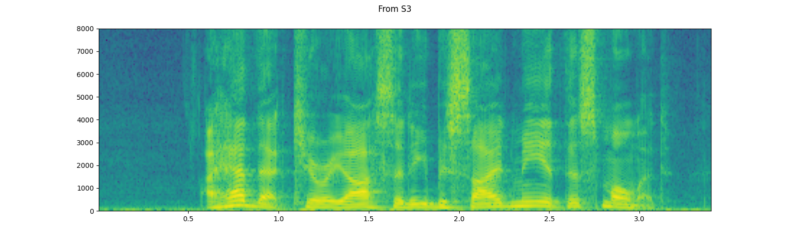
# Load audio from S3
client = boto3.client('s3', config=Config(signature_version=UNSIGNED))
response = client.get_object(Bucket=S3_BUCKET, Key=S3_KEY)
waveform, sample_rate = torchaudio.load(response['Body'])
plot_specgram(waveform, sample_rate, title="From S3")

• 
• 
• 

切片的技巧

提供 num_frames 和 frame_offset 參數將在解碼時對產生的張量物件進行切片。

可以使用常規的張量切片來實現相同的結果，（即 waveform[:, frame_offset:frame_offset+num_frames]），但是，提供 num_frames 和 frame_offset 參數效率更高。

這是因為一旦函數完成對請求的幀進行解碼，它就會停止資料擷取和解碼。當音訊資料通過網路傳輸時，這一點非常有利，因為一旦擷取到必要數量的資料，資料傳輸就會停止。

以下範例說明了這一點；

# Illustration of two different decoding methods.
# The first one will fetch all the data and decode them, while
# the second one will stop fetching data once it completes decoding.
# The resulting waveforms are identical.

frame_offset, num_frames = 16000, 16000  # Fetch and decode the 1 - 2 seconds

print("Fetching all the data...")
with requests.get(SAMPLE_WAV_SPEECH_URL, stream=True) as response:
  waveform1, sample_rate1 = torchaudio.load(response.raw)
  waveform1 = waveform1[:, frame_offset:frame_offset+num_frames]
  print(f" - Fetched {response.raw.tell()} bytes")

print("Fetching until the requested frames are available...")
with requests.get(SAMPLE_WAV_SPEECH_URL, stream=True) as response:
  waveform2, sample_rate2 = torchaudio.load(
      response.raw, frame_offset=frame_offset, num_frames=num_frames)
  print(f" - Fetched {response.raw.tell()} bytes")

print("Checking the resulting waveform ... ", end="")
assert (waveform1 == waveform2).all()
print("matched!")

輸出

Fetching all the data...
 - Fetched 108844 bytes
Fetching until the requested frames are available...
 - Fetched 65580 bytes
Checking the resulting waveform ... matched!

將音訊儲存至檔案

若要以常見應用程式可解讀的格式儲存音訊資料，您可以使用 torchaudio.save。

此函數接受類似路徑的物件和類似檔案的物件。

當傳遞類似檔案的物件時，您還需要提供 format 參數，以便函數知道應該使用哪種格式。如果是類似路徑的物件，函數將根據副檔名決定格式。如果您要儲存到沒有副檔名的檔案，則需要提供 format 參數。

以 WAV 格式儲存時，float32 Tensor 的預設編碼為 32 位元浮點 PCM。您可以提供 encoding 和 bits_per_sample 參數來更改此設定。例如，若要以 16 位元帶符號整數 PCM 儲存資料，您可以執行以下操作。

注意 以較低位元深度編碼儲存資料會減少產生的檔案大小，但會降低精度。

waveform, sample_rate = get_sample()
print_stats(waveform, sample_rate=sample_rate)

# Save without any encoding option.
# The function will pick up the encoding which
# the provided data fit
path = "save_example_default.wav"
torchaudio.save(path, waveform, sample_rate)
inspect_file(path)

# Save as 16-bit signed integer Linear PCM
# The resulting file occupies half the storage but loses precision
path = "save_example_PCM_S16.wav"
torchaudio.save(
    path, waveform, sample_rate,
    encoding="PCM_S", bits_per_sample=16)
inspect_file(path)

輸出

Sample Rate: 44100
Shape: (1, 109368)
Dtype: torch.float32
 - Max:      0.508
 - Min:     -0.449
 - Mean:    -0.000
 - Std Dev:  0.122

tensor([[0.0027, 0.0063, 0.0092,  ..., 0.0032, 0.0047, 0.0052]])

----------
Source: save_example_default.wav
----------
 - File size: 437530 bytes
 - AudioMetaData(sample_rate=44100, num_frames=109368, num_channels=1, bits_per_sample=32, encoding=PCM_F)
----------
Source: save_example_PCM_S16.wav
----------
 - File size: 218780 bytes
 - AudioMetaData(sample_rate=44100, num_frames=109368, num_channels=1, bits_per_sample=16, encoding=PCM_S)

torchaudio.save 也可以處理其他格式。舉幾個例子：

waveform, sample_rate = get_sample(resample=8000)

formats = [
  "mp3",
  "flac",
  "vorbis",
  "sph",
  "amb",
  "amr-nb",
  "gsm",
]

for format in formats:
  path = f"save_example.{format}"
  torchaudio.save(path, waveform, sample_rate, format=format)
  inspect_file(path)

輸出

----------
Source: save_example.mp3
----------
 - File size: 2664 bytes
 - AudioMetaData(sample_rate=8000, num_frames=21312, num_channels=1, bits_per_sample=0, encoding=MP3)
----------
Source: save_example.flac
----------
 - File size: 47315 bytes
 - AudioMetaData(sample_rate=8000, num_frames=19840, num_channels=1, bits_per_sample=24, encoding=FLAC)
----------
Source: save_example.vorbis
----------
 - File size: 9967 bytes
 - AudioMetaData(sample_rate=8000, num_frames=19840, num_channels=1, bits_per_sample=0, encoding=VORBIS)
----------
Source: save_example.sph
----------
 - File size: 80384 bytes
 - AudioMetaData(sample_rate=8000, num_frames=19840, num_channels=1, bits_per_sample=32, encoding=PCM_S)
----------
Source: save_example.amb
----------
 - File size: 79418 bytes
 - AudioMetaData(sample_rate=8000, num_frames=19840, num_channels=1, bits_per_sample=32, encoding=PCM_F)
----------
Source: save_example.amr-nb
----------
 - File size: 1618 bytes
 - AudioMetaData(sample_rate=8000, num_frames=19840, num_channels=1, bits_per_sample=0, encoding=AMR_NB)
----------
Source: save_example.gsm
----------
 - File size: 4092 bytes
 - AudioMetaData(sample_rate=8000, num_frames=0, num_channels=1, bits_per_sample=0, encoding=GSM)

儲存至類似檔案的物件

與其他輸入/輸出函數類似，您可以將音訊儲存到類似檔案的物件中。當儲存至類似檔案的物件時，需要使用 format 參數。

waveform, sample_rate = get_sample()

# Saving to Bytes buffer
buffer_ = io.BytesIO()
torchaudio.save(buffer_, waveform, sample_rate, format="wav")

buffer_.seek(0)
print(buffer_.read(16))

輸出

b'RIFF\x12\xad\x06\x00WAVEfmt '

重新取樣

若要將音訊波形從一個頻率重新取樣到另一個頻率，您可以使用 transforms.Resample 或 functional.resample。transforms.Resample 會預先計算並快取用於重新取樣的內核，而 functional.resample 則會動態計算，因此如果使用相同的參數重新取樣多個波形，使用 transforms.Resample 將會提高速度（請參閱基準測試部分）。

兩種重新取樣方法都使用 帶限正弦插值 來計算任意時間步長的訊號值。實作過程涉及卷積，因此我們可以利用 GPU/多線程來提升效能。當在多個子流程中使用重新取樣時，例如使用多個工作進程進行資料載入，您的應用程式可能會建立比系統可以有效處理的執行緒還要多。在這種情況下，設定 torch.set_num_threads(1) 可能會有幫助。

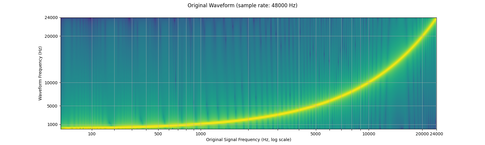
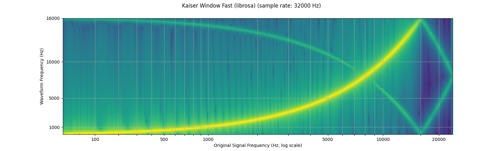
由於有限數量的樣本只能表示有限數量的頻率，因此重新取樣不會產生完美的結果，並且可以使用各種參數來控制其品質和計算速度。我們透過重新取樣對數正弦掃描來展示這些屬性，對數正弦掃描是一種隨時間呈指數增長的正弦波。

以下頻譜圖顯示了訊號的頻率表示，其中 x 軸標籤對應於原始波形的頻率（以對數刻度表示），y 軸對應於繪製波形的頻率，顏色強度表示振幅。

sample_rate = 48000
resample_rate = 32000

waveform = get_sine_sweep(sample_rate)
plot_sweep(waveform, sample_rate, title="Original Waveform")
play_audio(waveform, sample_rate)

resampler = T.Resample(sample_rate, resample_rate, dtype=waveform.dtype)
resampled_waveform = resampler(waveform)
plot_sweep(resampled_waveform, resample_rate, title="Resampled Waveform")
play_audio(waveform, sample_rate)

• 
• 

輸出

<IPython.lib.display.Audio object>
<IPython.lib.display.Audio object>

使用參數控制重新取樣品質

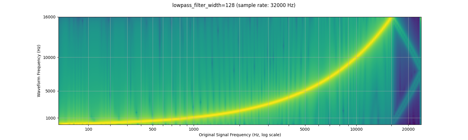
低通濾波器寬度

由於用於插值的濾波器是無限延伸的，因此 lowpass_filter_width 參數用於控制用於對插值進行窗口化的濾波器寬度。它也被稱為過零點數，因為插值在每個時間單位都會穿過零點。使用較大的 lowpass_filter_width 可以提供更清晰、更精確的濾波器，但計算成本也更高。

sample_rate = 48000
resample_rate = 32000

resampled_waveform = F.resample(waveform, sample_rate, resample_rate, lowpass_filter_width=6)
plot_sweep(resampled_waveform, resample_rate, title="lowpass_filter_width=6")

resampled_waveform = F.resample(waveform, sample_rate, resample_rate, lowpass_filter_width=128)
plot_sweep(resampled_waveform, resample_rate, title="lowpass_filter_width=128")

• 
• 

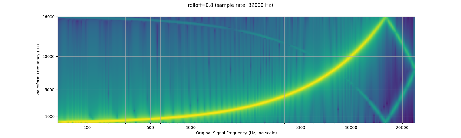
滾降

rolloff 參數表示為奈奎斯特頻率的分數，奈奎斯特頻率是由給定的有限取樣率可表示的最大頻率。rolloff 決定低通濾波器的截止頻率，並控制混疊的程度，混疊發生在高於奈奎斯特頻率的頻率被映射到較低頻率時。因此，較低的滾降將減少混疊量，但也會減少一些較高的頻率。

sample_rate = 48000
resample_rate = 32000

resampled_waveform = F.resample(waveform, sample_rate, resample_rate, rolloff=0.99)
plot_sweep(resampled_waveform, resample_rate, title="rolloff=0.99")

resampled_waveform = F.resample(waveform, sample_rate, resample_rate, rolloff=0.8)
plot_sweep(resampled_waveform, resample_rate, title="rolloff=0.8")

• 
• 

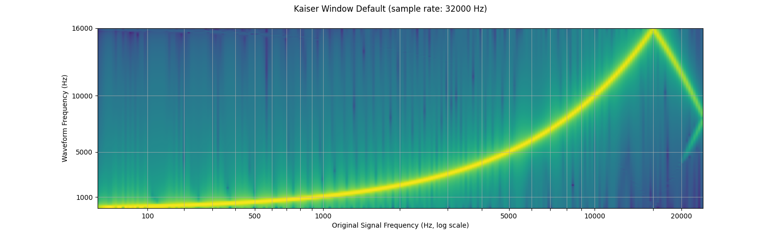
窗口函數

根據預設，torchaudio 的重新取樣使用漢明窗口濾波器，它是一個加權餘弦函數。它還支援凱澤窗口，這是一種接近最佳的窗口函數，它包含一個額外的 beta 參數，允許設計濾波器的平滑度和脈衝寬度。這可以使用 resampling_method 參數進行控制。

sample_rate = 48000
resample_rate = 32000

resampled_waveform = F.resample(waveform, sample_rate, resample_rate, resampling_method="sinc_interpolation")
plot_sweep(resampled_waveform, resample_rate, title="Hann Window Default")

resampled_waveform = F.resample(waveform, sample_rate, resample_rate, resampling_method="kaiser_window")
plot_sweep(resampled_waveform, resample_rate, title="Kaiser Window Default")

• 
• 

與 librosa 的比較

torchaudio 的重新取樣函數可用於產生與 librosa (resampy) 的凱澤窗口重新取樣類似的結果，但會有一些雜訊

sample_rate = 48000
resample_rate = 32000

### kaiser_best
resampled_waveform = F.resample(
    waveform,
    sample_rate,
    resample_rate,
    lowpass_filter_width=64,
    rolloff=0.9475937167399596,
    resampling_method="kaiser_window",
    beta=14.769656459379492
)
plot_sweep(resampled_waveform, resample_rate, title="Kaiser Window Best (torchaudio)")

librosa_resampled_waveform = torch.from_numpy(
    librosa.resample(waveform.squeeze().numpy(), sample_rate, resample_rate, res_type='kaiser_best')).unsqueeze(0)
plot_sweep(librosa_resampled_waveform, resample_rate, title="Kaiser Window Best (librosa)")

mse = torch.square(resampled_waveform - librosa_resampled_waveform).mean().item()
print("torchaudio and librosa kaiser best MSE:", mse)

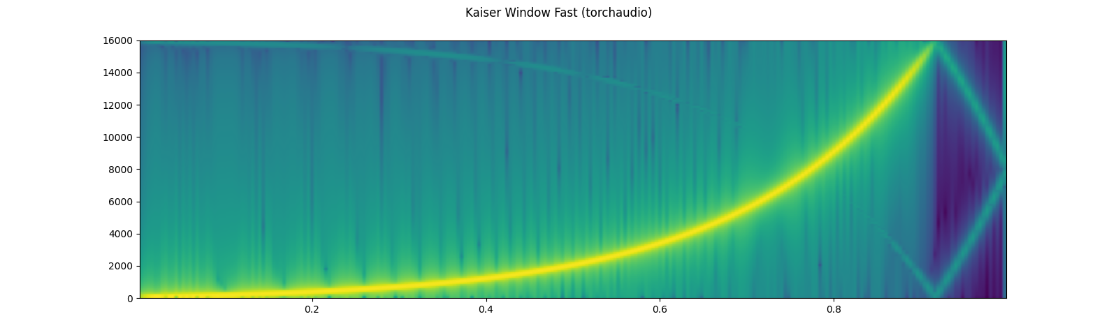
### kaiser_fast
resampled_waveform = F.resample(
    waveform,
    sample_rate,
    resample_rate,
    lowpass_filter_width=16,
    rolloff=0.85,
    resampling_method="kaiser_window",
    beta=8.555504641634386
)
plot_specgram(resampled_waveform, resample_rate, title="Kaiser Window Fast (torchaudio)")

librosa_resampled_waveform = torch.from_numpy(
    librosa.resample(waveform.squeeze().numpy(), sample_rate, resample_rate, res_type='kaiser_fast')).unsqueeze(0)
plot_sweep(librosa_resampled_waveform, resample_rate, title="Kaiser Window Fast (librosa)")

mse = torch.square(resampled_waveform - librosa_resampled_waveform).mean().item()
print("torchaudio and librosa kaiser fast MSE:", mse)

• 
• 
• 
• 

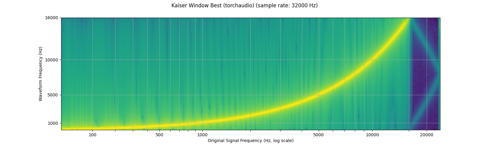
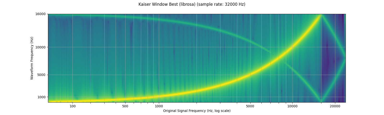
輸出

torchaudio and librosa kaiser best MSE: 2.080690115365992e-06
torchaudio and librosa kaiser fast MSE: 2.5200744248601027e-05

效能基準測試

以下是兩對取樣率之間波形降取樣和升取樣的基準測試。我們展示了 lowpass_filter_wdith、窗口類型和取樣率可能產生的效能影響。此外，我們還提供了與 librosa 的 kaiser_best 和 kaiser_fast 的比較，使用它們在 torchaudio 中的對應參數。

詳細說明結果

• 較大的 lowpass_filter_width 會導致更大的重新取樣內核，因此會增加內核計算和卷積的計算時間
• 使用 kaiser_window 的計算時間比預設的 sinc_interpolation 長，因為計算中間窗口值更為複雜 - 取樣率和重新取樣率之間較大的最大公因數將導致簡化，允許使用較小的內核和更快的內核計算。

configs = {
    "downsample (48 -> 44.1 kHz)": [48000, 44100],
    "downsample (16 -> 8 kHz)": [16000, 8000],
    "upsample (44.1 -> 48 kHz)": [44100, 48000],
    "upsample (8 -> 16 kHz)": [8000, 16000],
}

for label in configs:
  times, rows = [], []
  sample_rate = configs[label][0]
  resample_rate = configs[label][1]
  waveform = get_sine_sweep(sample_rate)

  # sinc 64 zero-crossings
  f_time = benchmark_resample("functional", waveform, sample_rate, resample_rate, lowpass_filter_width=64)
  t_time = benchmark_resample("transforms", waveform, sample_rate, resample_rate, lowpass_filter_width=64)
  times.append([None, 1000 * f_time, 1000 * t_time])
  rows.append(f"sinc (width 64)")

  # sinc 6 zero-crossings
  f_time = benchmark_resample("functional", waveform, sample_rate, resample_rate, lowpass_filter_width=16)
  t_time = benchmark_resample("transforms", waveform, sample_rate, resample_rate, lowpass_filter_width=16)
  times.append([None, 1000 * f_time, 1000 * t_time])
  rows.append(f"sinc (width 16)")

  # kaiser best
  lib_time = benchmark_resample("librosa", waveform, sample_rate, resample_rate, librosa_type="kaiser_best")
  f_time = benchmark_resample(
      "functional",
      waveform,
      sample_rate,
      resample_rate,
      lowpass_filter_width=64,
      rolloff=0.9475937167399596,
      resampling_method="kaiser_window",
      beta=14.769656459379492)
  t_time = benchmark_resample(
      "transforms",
      waveform,
      sample_rate,
      resample_rate,
      lowpass_filter_width=64,
      rolloff=0.9475937167399596,
      resampling_method="kaiser_window",
      beta=14.769656459379492)
  times.append([1000 * lib_time, 1000 * f_time, 1000 * t_time])
  rows.append(f"kaiser_best")

  # kaiser fast
  lib_time = benchmark_resample("librosa", waveform, sample_rate, resample_rate, librosa_type="kaiser_fast")
  f_time = benchmark_resample(
      "functional",
      waveform,
      sample_rate,
      resample_rate,
      lowpass_filter_width=16,
      rolloff=0.85,
      resampling_method="kaiser_window",
      beta=8.555504641634386)
  t_time = benchmark_resample(
      "transforms",
      waveform,
      sample_rate,
      resample_rate,
      lowpass_filter_width=16,
      rolloff=0.85,
      resampling_method="kaiser_window",
      beta=8.555504641634386)
  times.append([1000 * lib_time, 1000 * f_time, 1000 * t_time])
  rows.append(f"kaiser_fast")

  df = pd.DataFrame(times,
                    columns=["librosa", "functional", "transforms"],
                    index=rows)
  df.columns = pd.MultiIndex.from_product([[f"{label} time (ms)"],df.columns])
  display(df.round(2))

輸出

downsample (48 -> 44.1 kHz) time (ms)
                                              librosa functional transforms
sinc (width 64)                                   NaN      18.17       0.42
sinc (width 16)                                   NaN      16.67       0.37
kaiser_best                                     58.26      25.67       0.42
kaiser_fast                                      9.66      23.96       0.38
                downsample (16 -> 8 kHz) time (ms)
                                           librosa functional transforms
sinc (width 64)                                NaN       1.71       0.56
sinc (width 16)                                NaN       0.46       0.28
kaiser_best                                  20.48       0.94       0.52
kaiser_fast                                   4.26       0.56       0.28
                upsample (44.1 -> 48 kHz) time (ms)
                                            librosa functional transforms
sinc (width 64)                                 NaN      19.58       0.45
sinc (width 16)                                 NaN      18.19       0.42
kaiser_best                                   61.97      27.90       0.46
kaiser_fast                                    9.71      25.77       0.42
                upsample (8 -> 16 kHz) time (ms)
                                         librosa functional transforms
sinc (width 64)                              NaN       0.79       0.39
sinc (width 16)                              NaN       0.57       0.25
kaiser_best                                20.75       0.88       0.41
kaiser_fast                                 4.24       0.70       0.27

資料增強

torchaudio 提供了多種增強音訊資料的方法。

套用效果和濾波

torchaudio.sox_effects 模組提供了將 sox 命令之類的濾波器直接套用於 Tensor 物件和檔案物件音訊來源的方法。

有兩個函數可以做到這一點：

• torchaudio.sox_effects.apply_effects_tensor 用於將效果套用於 Tensor
• torchaudio.sox_effects.apply_effects_file 用於將效果套用於其他音訊來源

這兩個函數都採用 List[List[str]] 形式的效果。這與 sox 命令的工作方式基本一致，但需要注意的是，sox 命令會自動添加一些效果，而 torchaudio 的實作則不會。

有關可用效果的清單，請參閱 sox 文件。

提示 如果您需要動態載入和重新取樣音訊資料，則可以將 torchaudio.sox_effects.apply_effects_file 與 "rate" 效果一起使用。

注意 apply_effects_file 接受類似檔案的物件或類似路徑的物件。與 torchaudio.load 類似，當無法從檔案副檔名或標頭中檢測到音訊格式時，您可以提供 format 參數來告知音訊來源的格式。

注意 此過程不可微分。

# Load the data
waveform1, sample_rate1 = get_sample(resample=16000)

# Define effects
effects = [
  ["lowpass", "-1", "300"], # apply single-pole lowpass filter
  ["speed", "0.8"],  # reduce the speed
                     # This only changes sample rate, so it is necessary to
                     # add `rate` effect with original sample rate after this.
  ["rate", f"{sample_rate1}"],
  ["reverb", "-w"],  # Reverbration gives some dramatic feeling
]

# Apply effects
waveform2, sample_rate2 = torchaudio.sox_effects.apply_effects_tensor(
    waveform1, sample_rate1, effects)

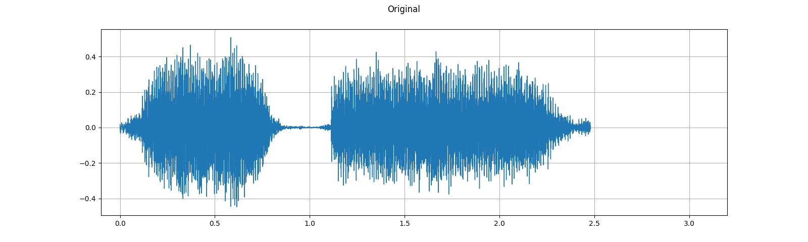
plot_waveform(waveform1, sample_rate1, title="Original", xlim=(-.1, 3.2))
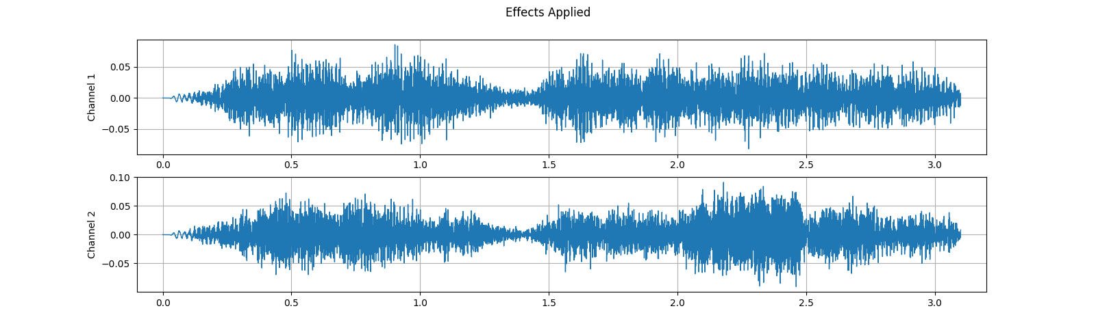
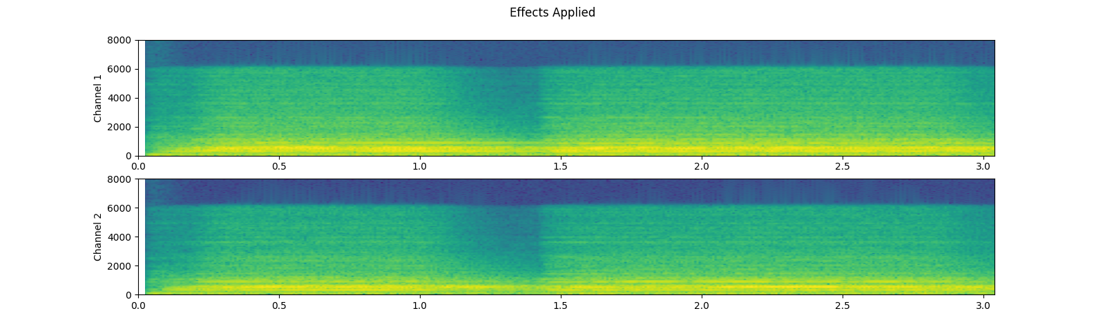
plot_waveform(waveform2, sample_rate2, title="Effects Applied", xlim=(-.1, 3.2))
print_stats(waveform1, sample_rate=sample_rate1, src="Original")
print_stats(waveform2, sample_rate=sample_rate2, src="Effects Applied")

• 
• 

輸出

----------
Source: Original
----------
Sample Rate: 16000
Shape: (1, 39680)
Dtype: torch.float32
 - Max:      0.507
 - Min:     -0.448
 - Mean:    -0.000
 - Std Dev:  0.122

tensor([[ 0.0007,  0.0076,  0.0122,  ..., -0.0049, -0.0025,  0.0020]])

----------
Source: Effects Applied
----------
Sample Rate: 16000
Shape: (2, 49600)
Dtype: torch.float32
 - Max:      0.091
 - Min:     -0.091
 - Mean:    -0.000
 - Std Dev:  0.021

tensor([[0.0000, 0.0000, 0.0000,  ..., 0.0069, 0.0058, 0.0045],
        [0.0000, 0.0000, 0.0000,  ..., 0.0085, 0.0085, 0.0085]])

請注意，套用效果後，影格數和通道數與原始的不同。讓我們聽聽音訊。聽起來是不是更有戲劇性？

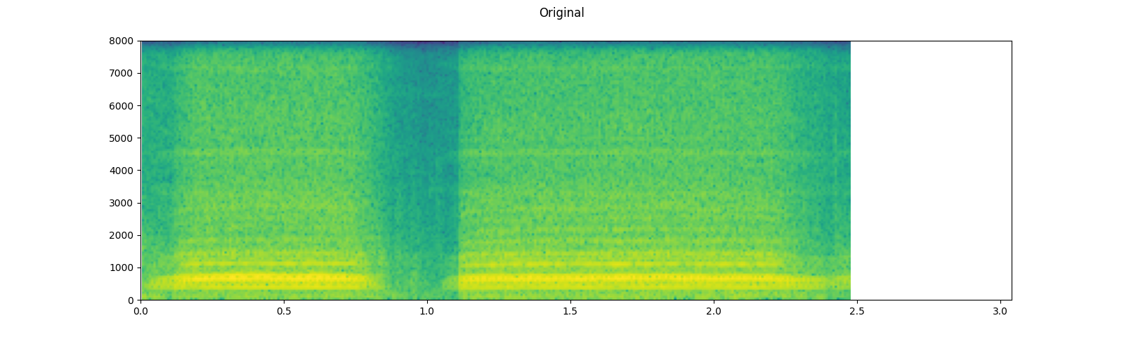
plot_specgram(waveform1, sample_rate1, title="Original", xlim=(0, 3.04))
play_audio(waveform1, sample_rate1)
plot_specgram(waveform2, sample_rate2, title="Effects Applied", xlim=(0, 3.04))
play_audio(waveform2, sample_rate2)

• 
• 

輸出

<IPython.lib.display.Audio object>
<IPython.lib.display.Audio object>

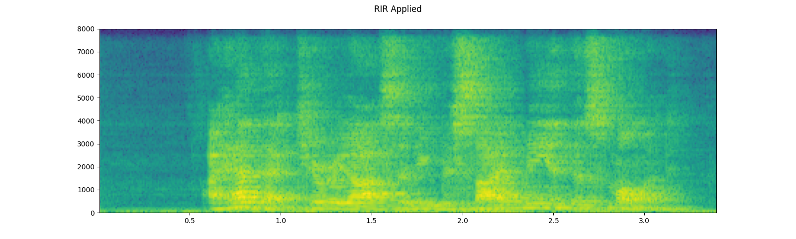
模擬房間混響

卷積混響 是一種用於使乾淨的音訊資料聽起來像在不同環境中的技術。

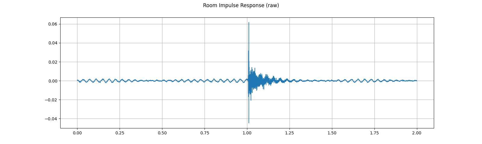
使用房間脈衝響應 (RIR)，我們可以使乾淨的語音聽起來像是在會議室中發出的。

對於這個過程，我們需要 RIR 資料。以下資料來自 VOiCES 資料集，但您可以自行錄製。只需打開麥克風並拍手即可。

sample_rate = 8000

rir_raw, _ = get_rir_sample(resample=sample_rate)

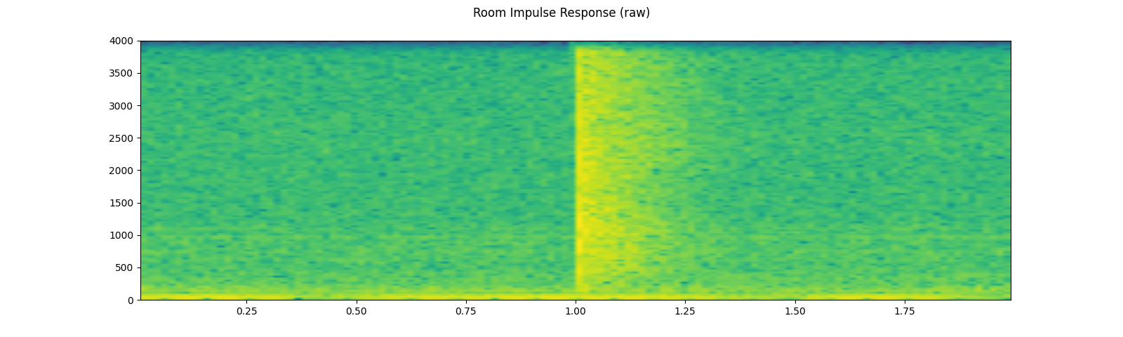
plot_waveform(rir_raw, sample_rate, title="Room Impulse Response (raw)", ylim=None)
plot_specgram(rir_raw, sample_rate, title="Room Impulse Response (raw)")
play_audio(rir_raw, sample_rate)

• 
• 

輸出

<IPython.lib.display.Audio object>

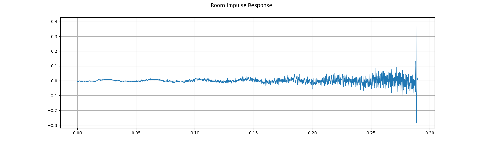
首先，我們需要清理 RIR。我們提取主要脈衝，將訊號功率標準化，然後翻轉時間軸。

rir = rir_raw[:, int(sample_rate*1.01):int(sample_rate*1.3)]
rir = rir / torch.norm(rir, p=2)
rir = torch.flip(rir, [1])

print_stats(rir)
plot_waveform(rir, sample_rate, title="Room Impulse Response", ylim=None)

輸出

Shape: (1, 2320)
Dtype: torch.float32
 - Max:      0.395
 - Min:     -0.286
 - Mean:    -0.000
 - Std Dev:  0.021

tensor([[-0.0052, -0.0076, -0.0071,  ...,  0.0184,  0.0173,  0.0070]])

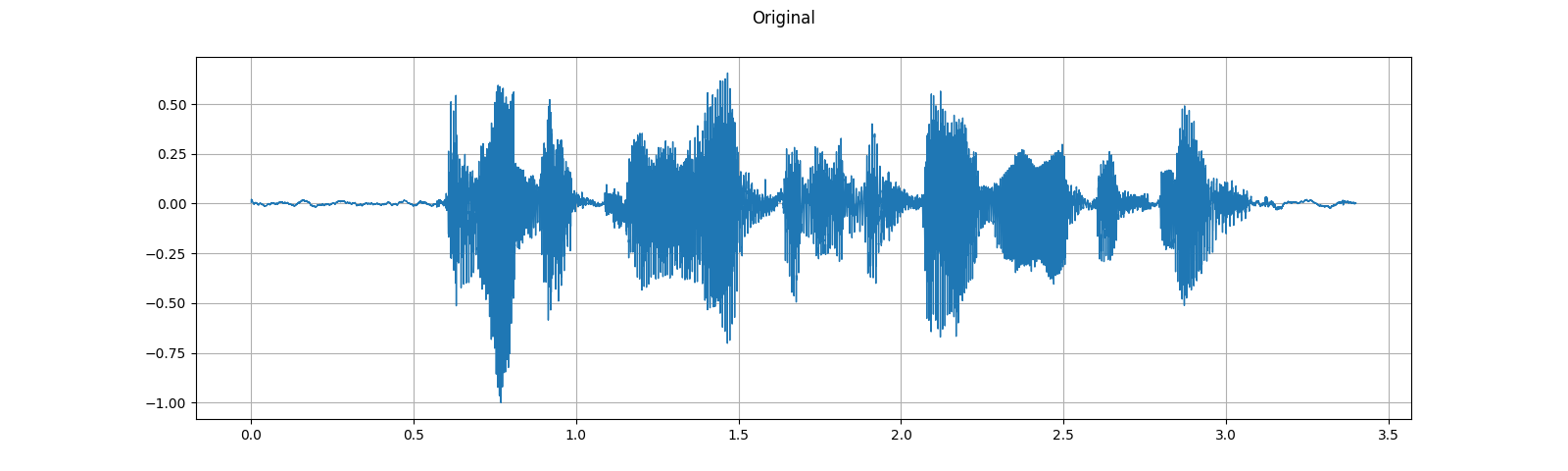
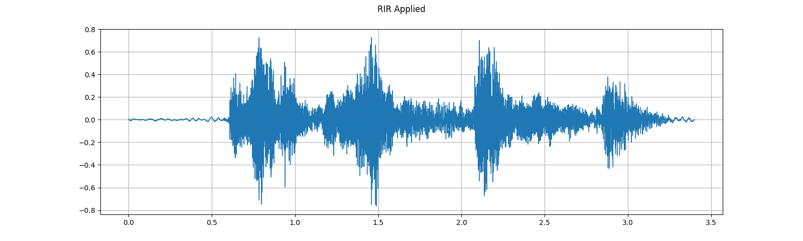
然後我們將語音訊號與 RIR 濾波器進行卷積。

speech, _ = get_speech_sample(resample=sample_rate)

speech_ = torch.nn.functional.pad(speech, (rir.shape[1]-1, 0))
augmented = torch.nn.functional.conv1d(speech_[None, ...], rir[None, ...])[0]

plot_waveform(speech, sample_rate, title="Original", ylim=None)
plot_waveform(augmented, sample_rate, title="RIR Applied", ylim=None)

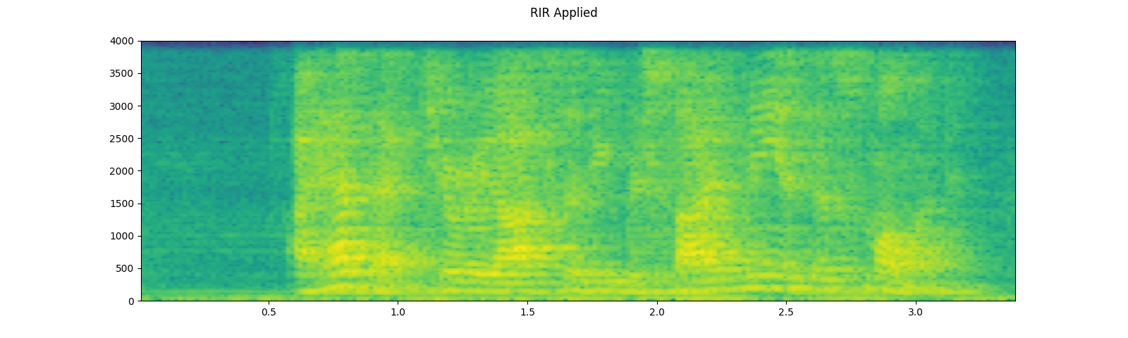
plot_specgram(speech, sample_rate, title="Original")
play_audio(speech, sample_rate)

plot_specgram(augmented, sample_rate, title="RIR Applied")
play_audio(augmented, sample_rate)

• 
• 
• 
• 

輸出

<IPython.lib.display.Audio object>
<IPython.lib.display.Audio object>

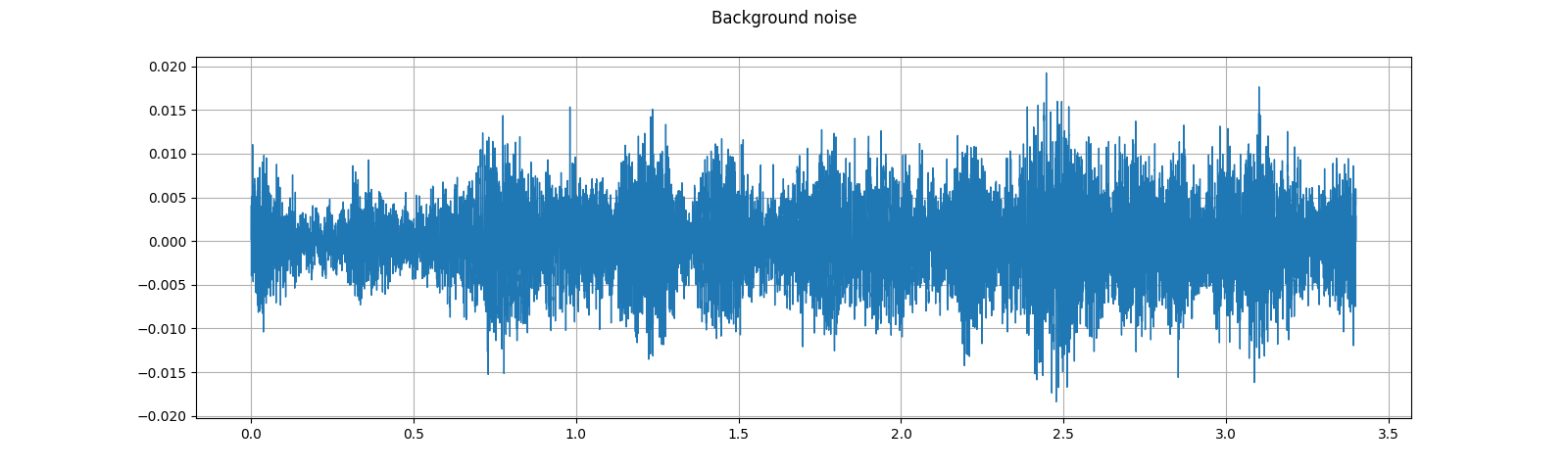
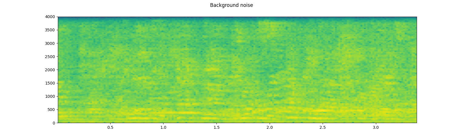
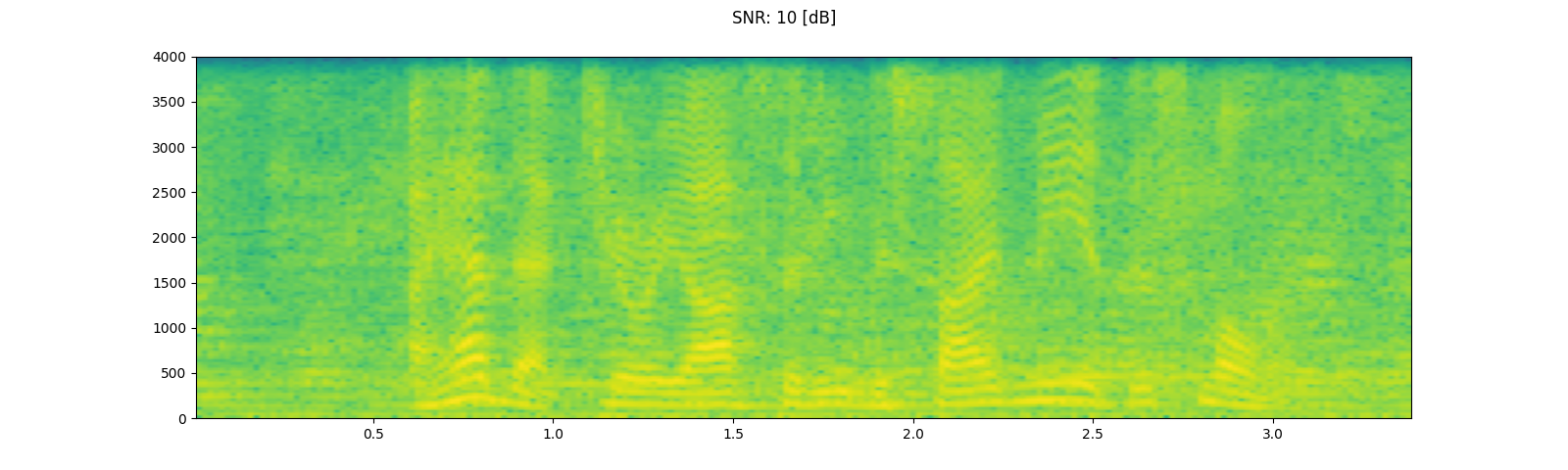
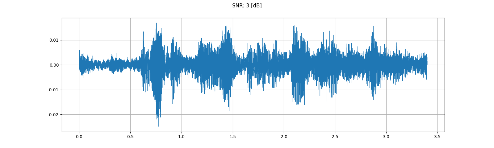
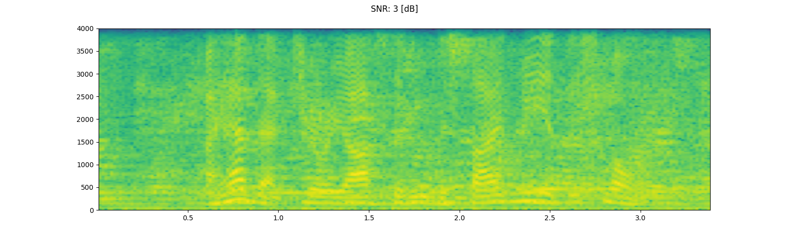
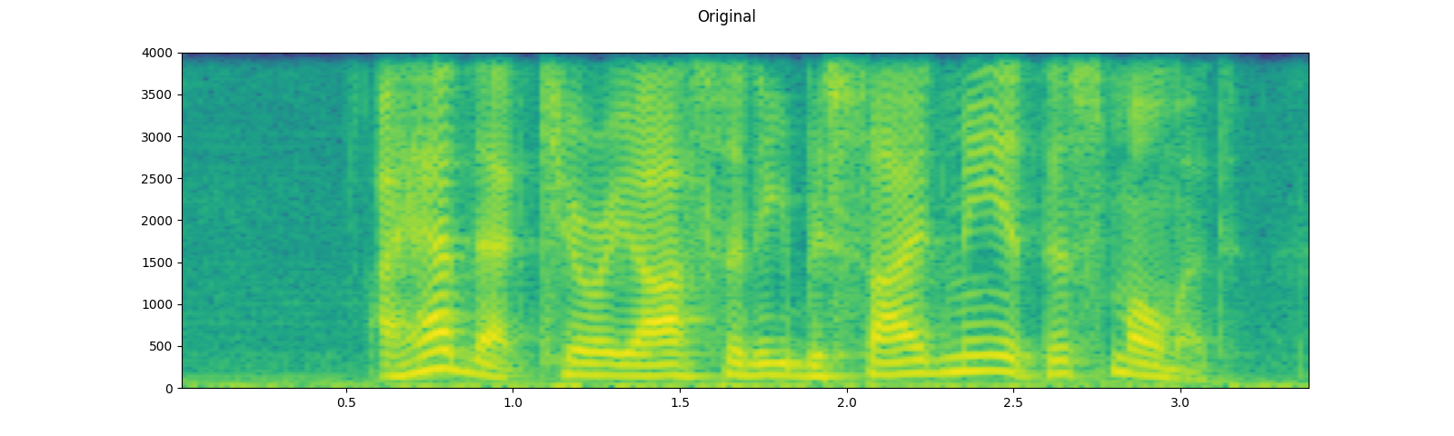
添加背景雜訊

若要將背景雜訊添加到音訊資料中，您只需添加音訊 Tensor 和雜訊 Tensor。調整雜訊強度的常用方法是更改訊號雜訊比 (SNR)。[維基百科]

\[\mathrm{SNR} = \frac{P_\mathrm{signal}}{P_\mathrm{noise}}\]

\[{\mathrm {SNR_{{dB}}}}=10\log _{{10}}\left({\mathrm {SNR}}\right)\]

sample_rate = 8000
speech, _ = get_speech_sample(resample=sample_rate)
noise, _ = get_noise_sample(resample=sample_rate)
noise = noise[:, :speech.shape[1]]

plot_waveform(noise, sample_rate, title="Background noise")
plot_specgram(noise, sample_rate, title="Background noise")
play_audio(noise, sample_rate)

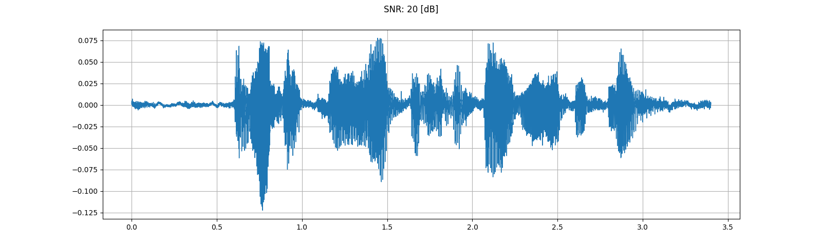
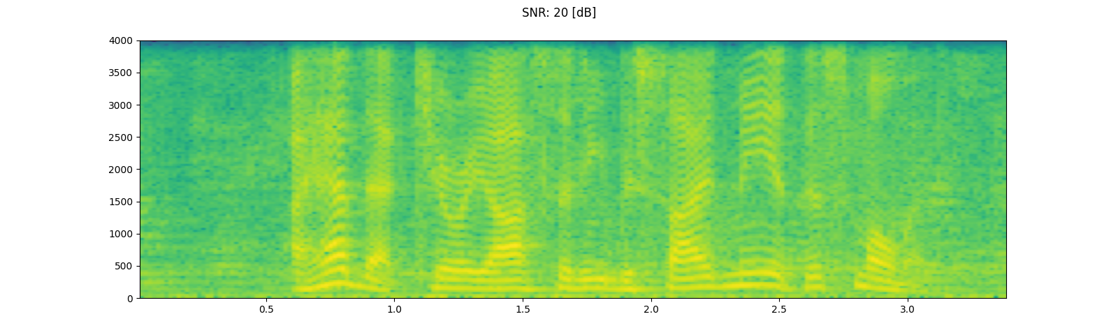
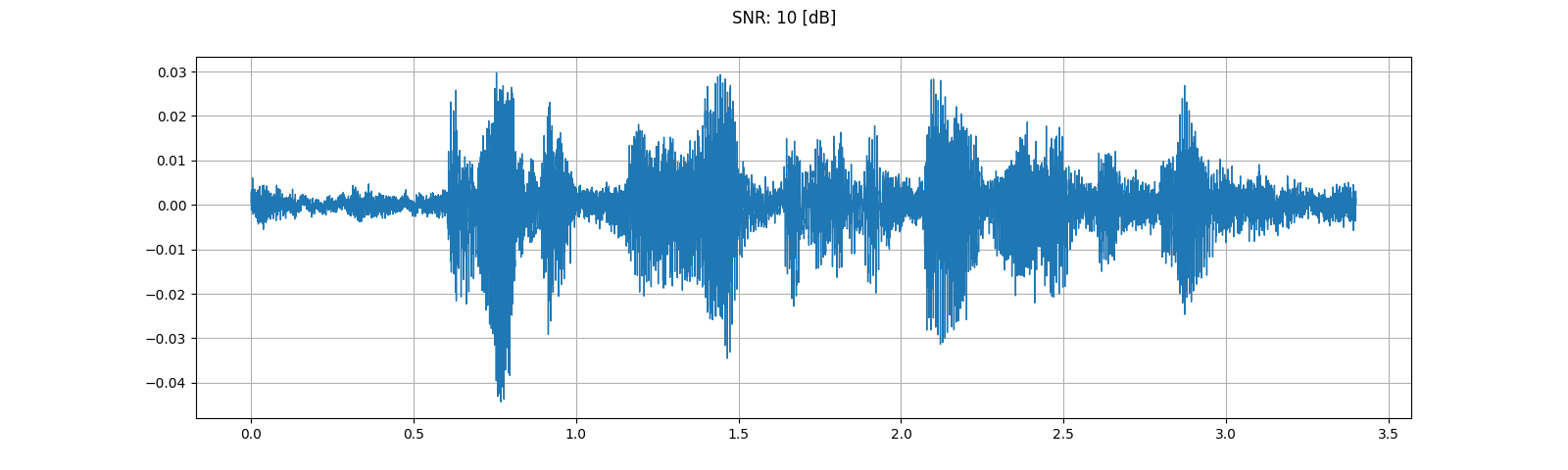
speech_power = speech.norm(p=2)
noise_power = noise.norm(p=2)

for snr_db in [20, 10, 3]:
  snr = math.exp(snr_db / 10)
  scale = snr * noise_power / speech_power
  noisy_speech = (scale * speech + noise) / 2

  plot_waveform(noisy_speech, sample_rate, title=f"SNR: {snr_db} [dB]")
  plot_specgram(noisy_speech, sample_rate, title=f"SNR: {snr_db} [dB]")
  play_audio(noisy_speech, sample_rate)

• 
• 
• 
• 
• 
• 
• 
• 

輸出

<IPython.lib.display.Audio object>
<IPython.lib.display.Audio object>
<IPython.lib.display.Audio object>
<IPython.lib.display.Audio object>

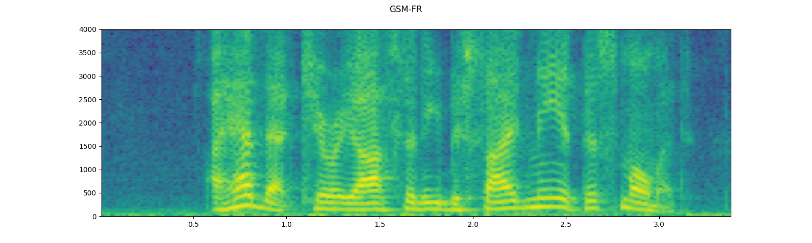
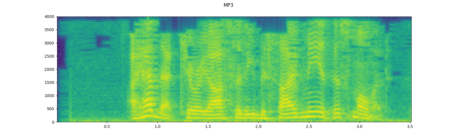
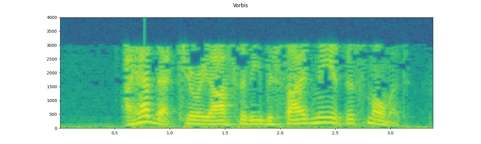
將編解碼器應用於 Tensor 物件

torchaudio.functional.apply_codec 可以將編解碼器應用於 Tensor 物件。

注意 此過程不可微分。

waveform, sample_rate = get_speech_sample(resample=8000)

plot_specgram(waveform, sample_rate, title="Original")
play_audio(waveform, sample_rate)

configs = [
    ({"format": "wav", "encoding": 'ULAW', "bits_per_sample": 8}, "8 bit mu-law"),
    ({"format": "gsm"}, "GSM-FR"),
    ({"format": "mp3", "compression": -9}, "MP3"),
    ({"format": "vorbis", "compression": -1}, "Vorbis"),
]
for param, title in configs:
  augmented = F.apply_codec(waveform, sample_rate, **param)
  plot_specgram(augmented, sample_rate, title=title)
  play_audio(augmented, sample_rate)

• 
• 
• 
• 
• 

輸出

<IPython.lib.display.Audio object>
<IPython.lib.display.Audio object>
<IPython.lib.display.Audio object>
<IPython.lib.display.Audio object>
<IPython.lib.display.Audio object>

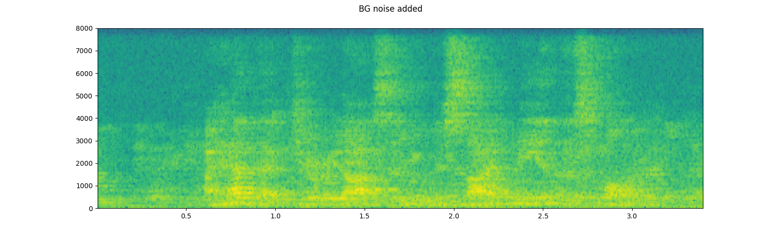
模擬電話錄音

結合前面的技術，我們可以模擬在回聲的房間裡，背景有人說話，一個人透過電話說話的音訊。

sample_rate = 16000
speech, _ = get_speech_sample(resample=sample_rate)

plot_specgram(speech, sample_rate, title="Original")
play_audio(speech, sample_rate)

# Apply RIR
rir, _ = get_rir_sample(resample=sample_rate, processed=True)
speech_ = torch.nn.functional.pad(speech, (rir.shape[1]-1, 0))
speech = torch.nn.functional.conv1d(speech_[None, ...], rir[None, ...])[0]

plot_specgram(speech, sample_rate, title="RIR Applied")
play_audio(speech, sample_rate)

# Add background noise
# Because the noise is recorded in the actual environment, we consider that
# the noise contains the acoustic feature of the environment. Therefore, we add
# the noise after RIR application.
noise, _ = get_noise_sample(resample=sample_rate)
noise = noise[:, :speech.shape[1]]

snr_db = 8
scale = math.exp(snr_db / 10) * noise.norm(p=2) / speech.norm(p=2)
speech = (scale * speech + noise) / 2

plot_specgram(speech, sample_rate, title="BG noise added")
play_audio(speech, sample_rate)

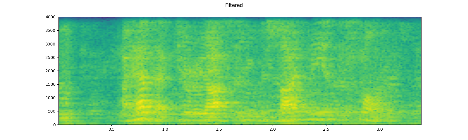
# Apply filtering and change sample rate
speech, sample_rate = torchaudio.sox_effects.apply_effects_tensor(
  speech,
  sample_rate,
  effects=[
      ["lowpass", "4000"],
      ["compand", "0.02,0.05", "-60,-60,-30,-10,-20,-8,-5,-8,-2,-8", "-8", "-7", "0.05"],
      ["rate", "8000"],
  ],
)

plot_specgram(speech, sample_rate, title="Filtered")
play_audio(speech, sample_rate)

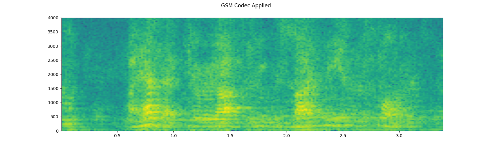
# Apply telephony codec
speech = F.apply_codec(speech, sample_rate, format="gsm")

plot_specgram(speech, sample_rate, title="GSM Codec Applied")
play_audio(speech, sample_rate)

• 
• 
• 
• 
• 

輸出

<IPython.lib.display.Audio object>
<IPython.lib.display.Audio object>
<IPython.lib.display.Audio object>
<IPython.lib.display.Audio object>
<IPython.lib.display.Audio object>

特徵提取

torchaudio 實作了音訊領域中常用的特徵提取。它們可在 torchaudio.functional 和 torchaudio.transforms 中使用。

functional 模組將特徵實作為獨立函數。它們是無狀態的。

transforms 模組以物件導向的方式實作特徵，使用 functional 和 torch.nn.Module 中的實作。

因為所有轉換都是 torch.nn.Module 的子類別，所以可以使用 TorchScript 對它們進行序列化。

如需可用功能的完整清單，請參閱說明文件。在本教學課程中，我們將探討時域和頻域之間的轉換（Spectrogram、GriffinLim、MelSpectrogram），以及稱為 SpecAugment 的增強技術。

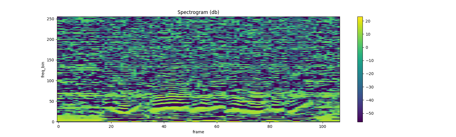
聲譜圖

若要取得音訊訊號的頻率表示，可以使用 Spectrogram 轉換。

waveform, sample_rate = get_speech_sample()

n_fft = 1024
win_length = None
hop_length = 512

# define transformation
spectrogram = T.Spectrogram(
    n_fft=n_fft,
    win_length=win_length,
    hop_length=hop_length,
    center=True,
    pad_mode="reflect",
    power=2.0,
)
# Perform transformation
spec = spectrogram(waveform)

print_stats(spec)
plot_spectrogram(spec[0], title='torchaudio')

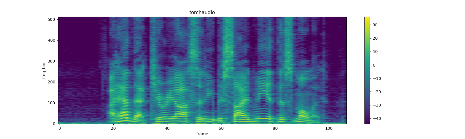
輸出

Shape: (1, 513, 107)
Dtype: torch.float32
 - Max:     4000.533
 - Min:      0.000
 - Mean:     5.726
 - Std Dev: 70.301

tensor([[[7.8743e+00, 4.4462e+00, 5.6781e-01,  ..., 2.7694e+01,
          8.9546e+00, 4.1289e+00],
         [7.1094e+00, 3.2595e+00, 7.3520e-01,  ..., 1.7141e+01,
          4.4812e+00, 8.0840e-01],
         [3.8374e+00, 8.2490e-01, 3.0779e-01,  ..., 1.8502e+00,
          1.1777e-01, 1.2369e-01],
         ...,
         [3.4708e-07, 1.0604e-05, 1.2395e-05,  ..., 7.4090e-06,
          8.2063e-07, 1.0176e-05],
         [4.7173e-05, 4.4329e-07, 3.9444e-05,  ..., 3.0622e-05,
          3.9735e-07, 8.1572e-06],
         [1.3221e-04, 1.6440e-05, 7.2536e-05,  ..., 5.4662e-05,
          1.1663e-05, 2.5758e-06]]])

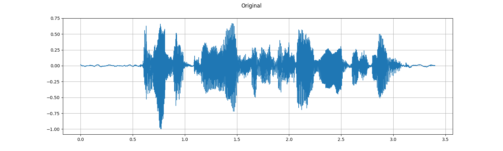
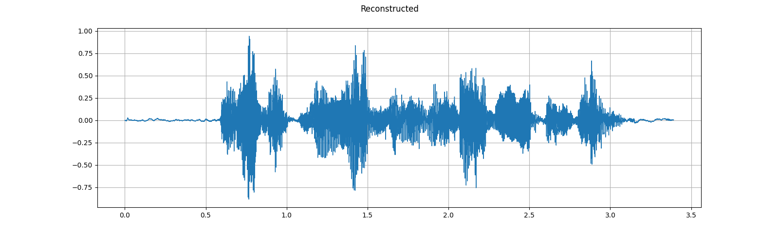
GriffinLim

若要從聲譜圖恢復波形，可以使用 GriffinLim。

torch.random.manual_seed(0)
waveform, sample_rate = get_speech_sample()
plot_waveform(waveform, sample_rate, title="Original")
play_audio(waveform, sample_rate)

n_fft = 1024
win_length = None
hop_length = 512

spec = T.Spectrogram(
    n_fft=n_fft,
    win_length=win_length,
    hop_length=hop_length,
)(waveform)

griffin_lim = T.GriffinLim(
    n_fft=n_fft,
    win_length=win_length,
    hop_length=hop_length,
)
waveform = griffin_lim(spec)

plot_waveform(waveform, sample_rate, title="Reconstructed")
play_audio(waveform, sample_rate)

• 
• 

輸出

<IPython.lib.display.Audio object>
<IPython.lib.display.Audio object>

梅爾濾波器組

torchaudio.functional.create_fb_matrix 可以產生濾波器組，將頻率區間轉換為梅爾尺度區間。

由於此函數不需要輸入音訊/特徵，因此在 torchaudio.transforms 中沒有對應的轉換。

n_fft = 256
n_mels = 64
sample_rate = 6000

mel_filters = F.create_fb_matrix(
    int(n_fft // 2 + 1),
    n_mels=n_mels,
    f_min=0.,
    f_max=sample_rate/2.,
    sample_rate=sample_rate,
    norm='slaney'
)
plot_mel_fbank(mel_filters, "Mel Filter Bank - torchaudio")

與 librosa 的比較

作為比較，以下是以 librosa 取得梅爾濾波器組的對應方法。

mel_filters_librosa = librosa.filters.mel(
    sample_rate,
    n_fft,
    n_mels=n_mels,
    fmin=0.,
    fmax=sample_rate/2.,
    norm='slaney',
    htk=True,
).T

plot_mel_fbank(mel_filters_librosa, "Mel Filter Bank - librosa")

mse = torch.square(mel_filters - mel_filters_librosa).mean().item()
print('Mean Square Difference: ', mse)

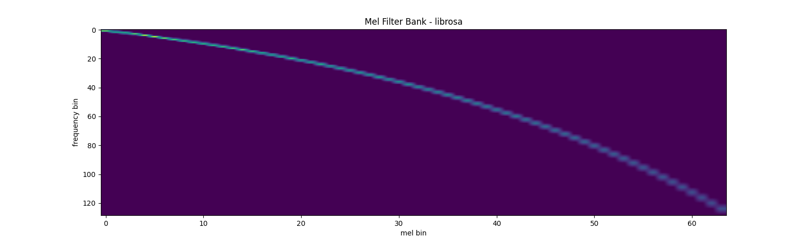
輸出

Mean Square Difference:  3.795462323290159e-17

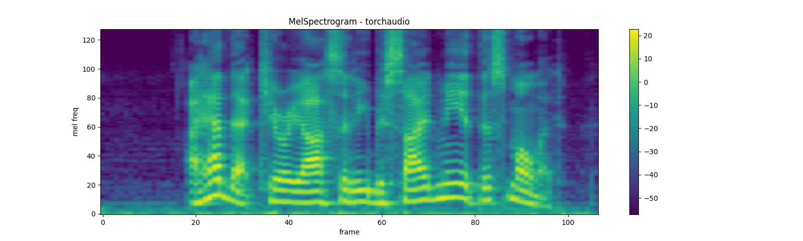
梅爾頻譜圖

梅爾尺度聲譜圖是聲譜圖和梅爾尺度轉換的組合。在 torchaudio 中，有一個轉換 MelSpectrogram，它由 Spectrogram 和 MelScale 組成。

waveform, sample_rate = get_speech_sample()

n_fft = 1024
win_length = None
hop_length = 512
n_mels = 128

mel_spectrogram = T.MelSpectrogram(
    sample_rate=sample_rate,
    n_fft=n_fft,
    win_length=win_length,
    hop_length=hop_length,
    center=True,
    pad_mode="reflect",
    power=2.0,
    norm='slaney',
    onesided=True,
    n_mels=n_mels,
    mel_scale="htk",
)

melspec = mel_spectrogram(waveform)
plot_spectrogram(
    melspec[0], title="MelSpectrogram - torchaudio", ylabel='mel freq')

與 librosa 的比較

作為比較，以下是以 librosa 取得梅爾尺度聲譜圖的對應方法。

melspec_librosa = librosa.feature.melspectrogram(
    waveform.numpy()[0],
    sr=sample_rate,
    n_fft=n_fft,
    hop_length=hop_length,
    win_length=win_length,
    center=True,
    pad_mode="reflect",
    power=2.0,
    n_mels=n_mels,
    norm='slaney',
    htk=True,
)
plot_spectrogram(
    melspec_librosa, title="MelSpectrogram - librosa", ylabel='mel freq')

mse = torch.square(melspec - melspec_librosa).mean().item()
print('Mean Square Difference: ', mse)

輸出

Mean Square Difference:  1.17573561997375e-10

MFCC

waveform, sample_rate = get_speech_sample()

n_fft = 2048
win_length = None
hop_length = 512
n_mels = 256
n_mfcc = 256

mfcc_transform = T.MFCC(
    sample_rate=sample_rate,
    n_mfcc=n_mfcc,
    melkwargs={
      'n_fft': n_fft,
      'n_mels': n_mels,
      'hop_length': hop_length,
      'mel_scale': 'htk',
    }
)

mfcc = mfcc_transform(waveform)

plot_spectrogram(mfcc[0])

與 librosa 的比較

melspec = librosa.feature.melspectrogram(
  y=waveform.numpy()[0], sr=sample_rate, n_fft=n_fft,
  win_length=win_length, hop_length=hop_length,
  n_mels=n_mels, htk=True, norm=None)

mfcc_librosa = librosa.feature.mfcc(
  S=librosa.core.spectrum.power_to_db(melspec),
  n_mfcc=n_mfcc, dct_type=2, norm='ortho')

plot_spectrogram(mfcc_librosa)

mse = torch.square(mfcc - mfcc_librosa).mean().item()
print('Mean Square Difference: ', mse)

輸出

Mean Square Difference:  4.258112085153698e-08

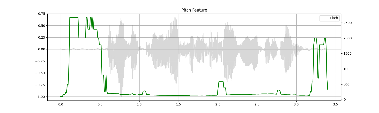
音高

waveform, sample_rate = get_speech_sample()

pitch = F.detect_pitch_frequency(waveform, sample_rate)
plot_pitch(waveform, sample_rate, pitch)
play_audio(waveform, sample_rate)

輸出

<IPython.lib.display.Audio object>

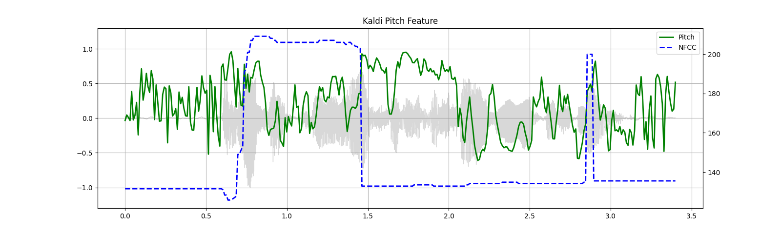
Kaldi 音高（測試版）

Kaldi 音高特徵 [1] 是針對 ASR 應用程式調整的音高偵測機制。這是 torchaudio 中的測試版功能，並且僅提供 functional 形式。

1. 針對自動語音辨識調整的音高提取演算法

   Ghahremani、B. BabaAli、D. Povey、K. Riedhammer、J. Trmal 和 S. Khudanpur

   2014 年 IEEE 聲學、語音和訊號處理國際會議 (ICASSP)，佛羅倫斯，2014 年，第 2494-2498 頁，doi: 10.1109/ICASSP.2014.6854049。[摘要]、[論文]

waveform, sample_rate = get_speech_sample(resample=16000)

pitch_feature = F.compute_kaldi_pitch(waveform, sample_rate)
pitch, nfcc = pitch_feature[..., 0], pitch_feature[..., 1]

plot_kaldi_pitch(waveform, sample_rate, pitch, nfcc)
play_audio(waveform, sample_rate)

輸出

<IPython.lib.display.Audio object>

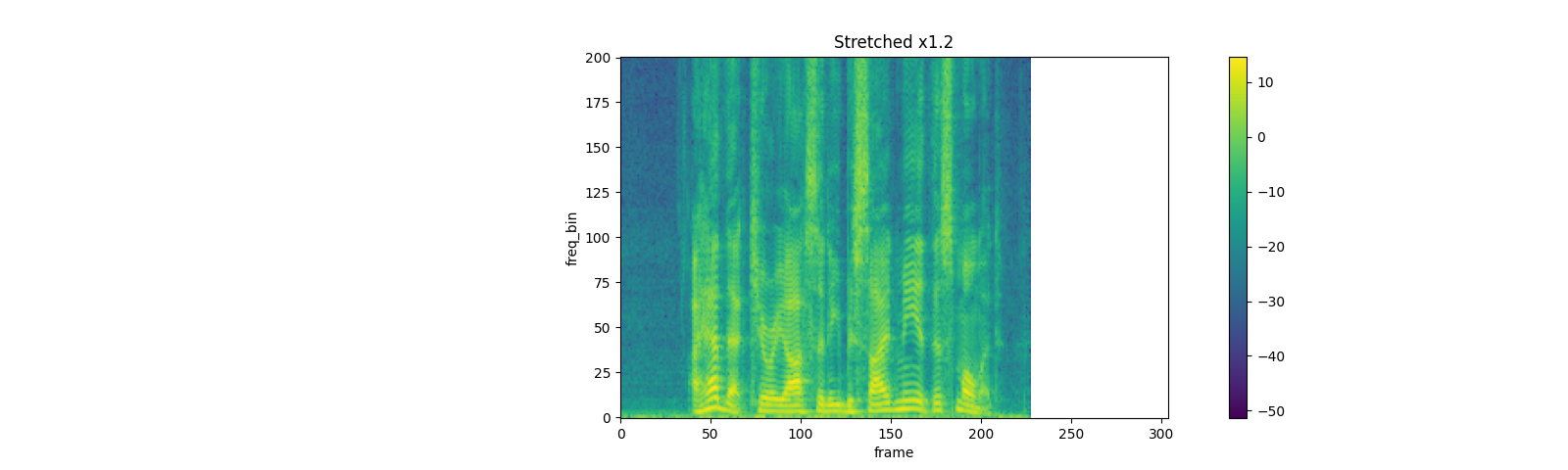
特徵增強

SpecAugment

SpecAugment 是一種流行的增強技術，應用於聲譜圖。

torchaudio 實作了 TimeStrech、TimeMasking 和 FrequencyMasking。

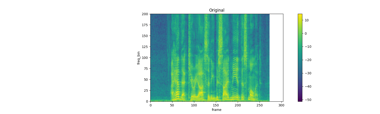
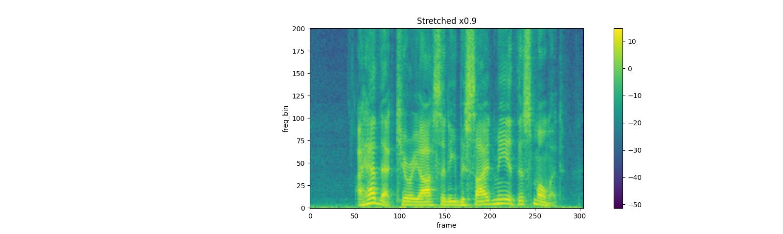
TimeStrech

spec = get_spectrogram(power=None)
strech = T.TimeStretch()

rate = 1.2
spec_ = strech(spec, rate)
plot_spectrogram(spec_[0].abs(), title=f"Stretched x{rate}", aspect='equal', xmax=304)

plot_spectrogram(spec[0].abs(), title="Original", aspect='equal', xmax=304)

rate = 0.9
spec_ = strech(spec, rate)
plot_spectrogram(spec_[0].abs(), title=f"Stretched x{rate}", aspect='equal', xmax=304)

• 
• 
• 

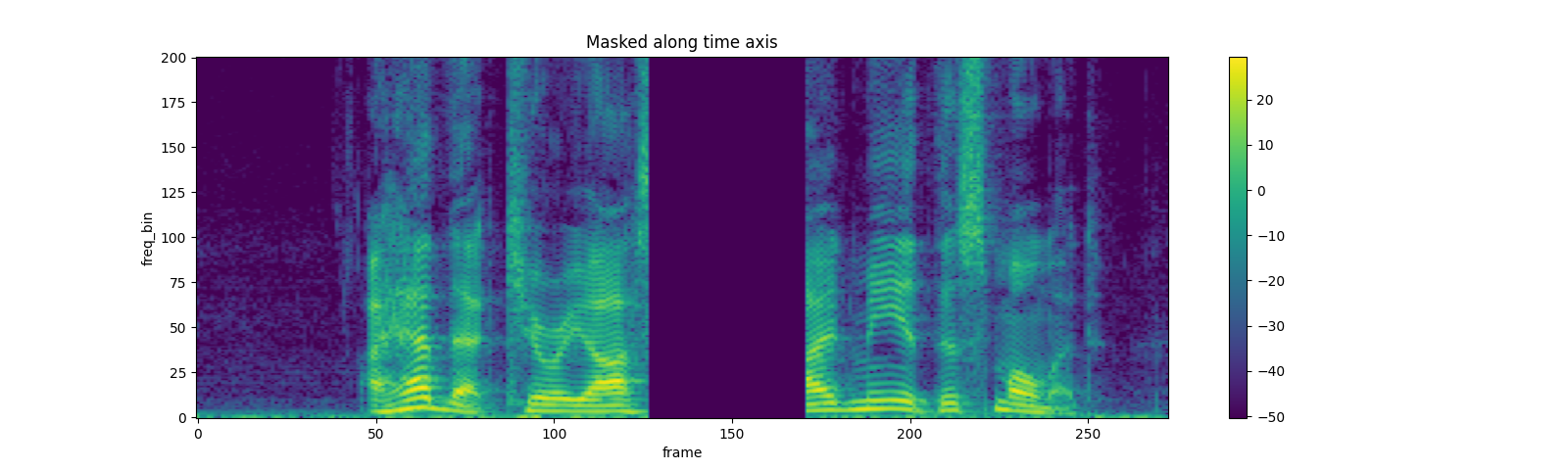
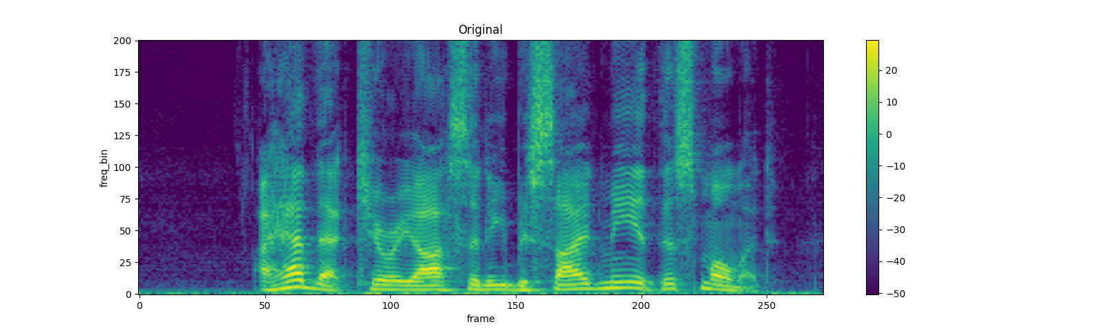
TimeMasking

torch.random.manual_seed(4)

spec = get_spectrogram()
plot_spectrogram(spec[0], title="Original")

masking = T.TimeMasking(time_mask_param=80)
spec = masking(spec)

plot_spectrogram(spec[0], title="Masked along time axis")

• 
• 

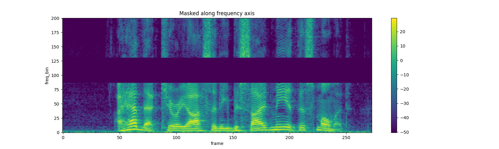
FrequencyMasking

torch.random.manual_seed(4)

spec = get_spectrogram()
plot_spectrogram(spec[0], title="Original")

masking = T.FrequencyMasking(freq_mask_param=80)
spec = masking(spec)

plot_spectrogram(spec[0], title="Masked along frequency axis")

• 
• 

資料集

torchaudio 提供對常見、公開資料集的輕鬆存取。請查看官方文件以取得可用資料集的清單。

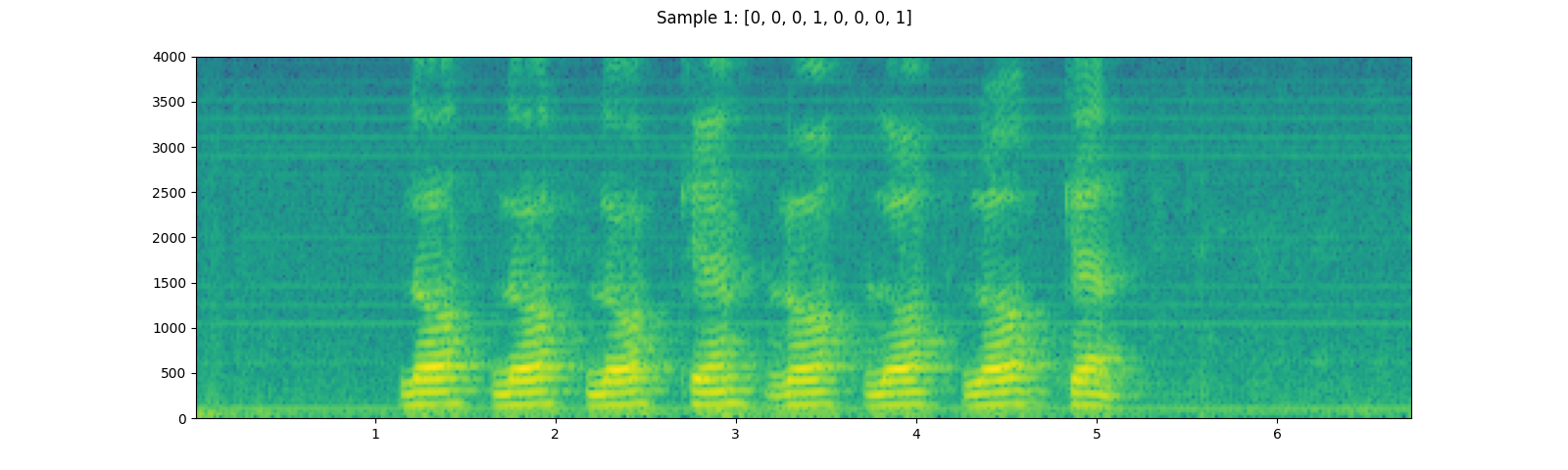
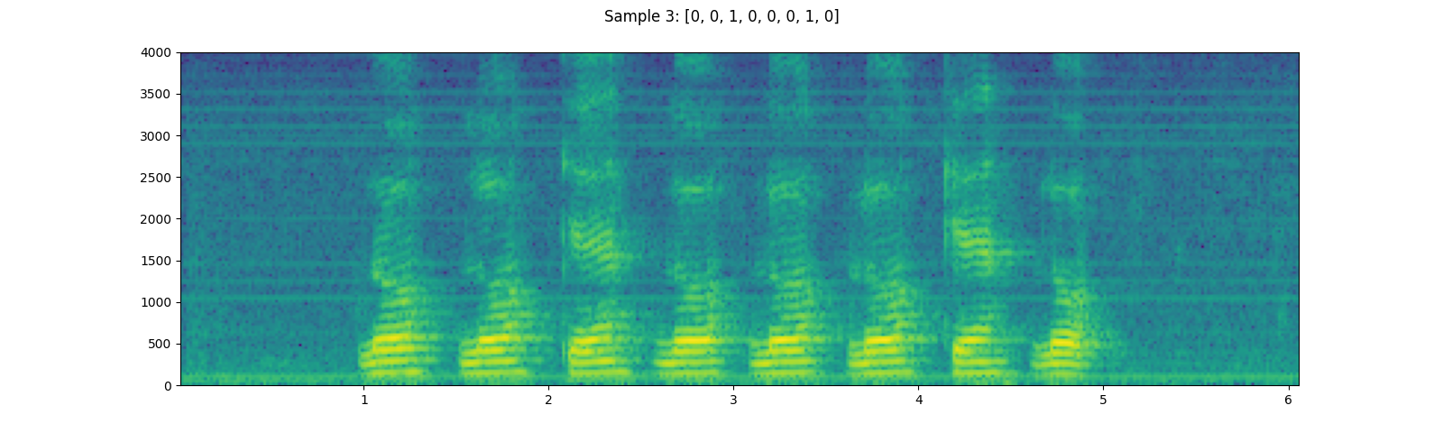
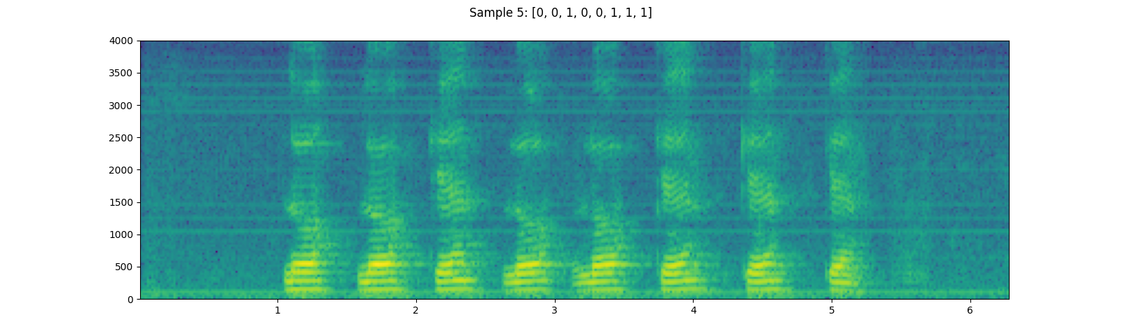
在這裡，我們以 YESNO 資料集為例，看看如何使用它。

YESNO_DOWNLOAD_PROCESS.join()

dataset = torchaudio.datasets.YESNO(YESNO_DATASET_PATH, download=True)

for i in [1, 3, 5]:
  waveform, sample_rate, label = dataset[i]
  plot_specgram(waveform, sample_rate, title=f"Sample {i}: {label}")
  play_audio(waveform, sample_rate)

• 
• 
• 

輸出

<IPython.lib.display.Audio object>
<IPython.lib.display.Audio object>
<IPython.lib.display.Audio object>