注意

點擊此處下載完整的範例程式碼

TorchVision 物件偵測微調教程¶

建立於：2023 年 12 月 14 日 | 最後更新：2024 年 6 月 11 日 | 最後驗證：2024 年 11 月 05 日

在本教程中，我們將在 Penn-Fudan 行人偵測和分割資料庫上微調預訓練的 Mask R-CNN 模型。它包含 170 張影像，其中包含 345 個行人實例，我們將使用它來說明如何使用 torchvision 中的新功能，以便在自定義資料集上訓練物件偵測和實例分割模型。

注意

本教程僅適用於 torchvision 版本 >=0.16 或 nightly 版本。如果您使用的是 torchvision<=0.15，請改為遵循本教程。

定義資料集¶

用於訓練物件偵測、實例分割和人物關鍵點偵測的參考腳本允許輕鬆支援添加新的自定義資料集。資料集應繼承自標準 torch.utils.data.Dataset 類別，並實作 __len__ 和 __getitem__。

我們唯一需要的特殊性是資料集 __getitem__ 應該返回一個元組

image: 形狀為 [3, H, W] 的 torchvision.tv_tensors.Image，一個純張量，或大小為 (H, W) 的 PIL 影像
target: 包含以下欄位的字典
- boxes, 形狀為 [N, 4] 的 torchvision.tv_tensors.BoundingBoxes：N 個邊界框的座標，格式為 [x0, y0, x1, y1]，範圍從 0 到 W 和 0 到 H
- labels, 形狀為 [N] 的整數 torch.Tensor：每個邊界框的標籤。0 始終代表背景類別。
- image_id, int: 影像識別碼。它在資料集中的所有影像之間應該是唯一的，並在評估期間使用
- area, 形狀為 [N] 的浮點數 torch.Tensor：邊界框的面積。這用於使用 COCO 指標進行評估，以區分小型、中型和大型框之間的指標分數。
- iscrowd, uint8 類型的 torch.Tensor，形狀為 [N]：在評估期間，iscrowd=True 的實例將會被忽略。
- (可選) masks, torchvision.tv_tensors.Mask 類型的物件，形狀為 [N, H, W]：每個物件的分割遮罩。

如果您的資料集符合以上需求，那麼它將適用於參考腳本中的訓練和評估程式碼。評估程式碼將使用 pycocotools 中的腳本，可以使用 pip install pycocotools 安裝。

注意

對於 Windows 系統，請使用以下命令從 gautamchitnis 安裝 pycocotools：

pip install git+https://github.com/gautamchitnis/cocoapi.git@cocodataset-master#subdirectory=PythonAPI

關於 labels 的一點說明。該模型將類別 0 視為背景。如果您的資料集不包含背景類別，則您的 labels 中不應包含 0。例如，假設您只有兩個類別，cat 和 dog，您可以定義 1 (不是 0) 來表示 cats，並定義 2 來表示 dogs。因此，舉例來說，如果其中一個圖像同時具有這兩個類別，則您的 labels tensor 應該看起來像 [1, 2]。

此外，如果您想在訓練期間使用長寬比分組（以便每個批次僅包含具有相似長寬比的圖像），建議您也實現一個 get_height_and_width 方法，該方法返回圖像的高度和寬度。如果未提供此方法，我們將通過 __getitem__ 查詢資料集的所有元素，這會將圖像載入記憶體中，並且比提供自定義方法慢。

為 PennFudan 撰寫自定義資料集¶

讓我們為 PennFudan 資料集編寫一個資料集。首先，讓我們下載資料集並解壓縮 zip 檔案

wget https://www.cis.upenn.edu/~jshi/ped_html/PennFudanPed.zip -P data
cd data && unzip PennFudanPed.zip

我們有以下文件夾結構

PennFudanPed/
  PedMasks/
    FudanPed00001_mask.png
    FudanPed00002_mask.png
    FudanPed00003_mask.png
    FudanPed00004_mask.png
    ...
  PNGImages/
    FudanPed00001.png
    FudanPed00002.png
    FudanPed00003.png
    FudanPed00004.png

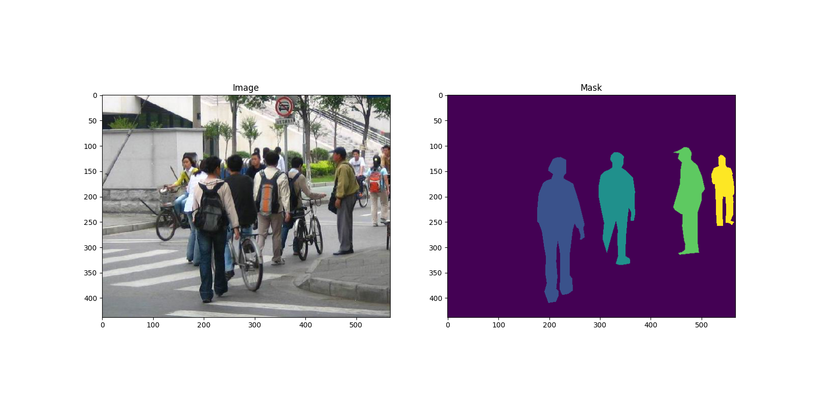
這是一個圖像和分割遮罩對的例子

import matplotlib.pyplot as plt
from torchvision.io import read_image


image = read_image("data/PennFudanPed/PNGImages/FudanPed00046.png")
mask = read_image("data/PennFudanPed/PedMasks/FudanPed00046_mask.png")

plt.figure(figsize=(16, 8))
plt.subplot(121)
plt.title("Image")
plt.imshow(image.permute(1, 2, 0))
plt.subplot(122)
plt.title("Mask")
plt.imshow(mask.permute(1, 2, 0))

<matplotlib.image.AxesImage object at 0x7f36917736a0>

因此，每個圖像都有一個相應的分割遮罩，其中每種顏色對應於不同的實例。讓我們為這個資料集編寫一個 torch.utils.data.Dataset 類別。在下面的程式碼中，我們將圖像、邊界框和遮罩包裝到 torchvision.tv_tensors.TVTensor 類別中，以便我們可以為給定的物件檢測和分割任務應用 torchvision 內建的轉換 (新的 Transforms API)。也就是說，圖像 tensor 將被 torchvision.tv_tensors.Image 包裝，邊界框被 torchvision.tv_tensors.BoundingBoxes 包裝，遮罩被 torchvision.tv_tensors.Mask 包裝。由於 torchvision.tv_tensors.TVTensor 是 torch.Tensor 的子類別，因此包裝的物件也是 tensor，並繼承了普通的 torch.Tensor API。關於 torchvision tv_tensors 的更多信息，請參閱此文件。

import os
import torch

from torchvision.io import read_image
from torchvision.ops.boxes import masks_to_boxes
from torchvision import tv_tensors
from torchvision.transforms.v2 import functional as F


class PennFudanDataset(torch.utils.data.Dataset):
    def __init__(self, root, transforms):
        self.root = root
        self.transforms = transforms
        # load all image files, sorting them to
        # ensure that they are aligned
        self.imgs = list(sorted(os.listdir(os.path.join(root, "PNGImages"))))
        self.masks = list(sorted(os.listdir(os.path.join(root, "PedMasks"))))

    def __getitem__(self, idx):
        # load images and masks
        img_path = os.path.join(self.root, "PNGImages", self.imgs[idx])
        mask_path = os.path.join(self.root, "PedMasks", self.masks[idx])
        img = read_image(img_path)
        mask = read_image(mask_path)
        # instances are encoded as different colors
        obj_ids = torch.unique(mask)
        # first id is the background, so remove it
        obj_ids = obj_ids[1:]
        num_objs = len(obj_ids)

        # split the color-encoded mask into a set
        # of binary masks
        masks = (mask == obj_ids[:, None, None]).to(dtype=torch.uint8)

        # get bounding box coordinates for each mask
        boxes = masks_to_boxes(masks)

        # there is only one class
        labels = torch.ones((num_objs,), dtype=torch.int64)

        image_id = idx
        area = (boxes[:, 3] - boxes[:, 1]) * (boxes[:, 2] - boxes[:, 0])
        # suppose all instances are not crowd
        iscrowd = torch.zeros((num_objs,), dtype=torch.int64)

        # Wrap sample and targets into torchvision tv_tensors:
        img = tv_tensors.Image(img)

        target = {}
        target["boxes"] = tv_tensors.BoundingBoxes(boxes, format="XYXY", canvas_size=F.get_size(img))
        target["masks"] = tv_tensors.Mask(masks)
        target["labels"] = labels
        target["image_id"] = image_id
        target["area"] = area
        target["iscrowd"] = iscrowd

        if self.transforms is not None:
            img, target = self.transforms(img, target)

        return img, target

    def __len__(self):
        return len(self.imgs)

這就是資料集的全部內容。現在讓我們定義一個可以在此資料集上執行預測的模型。

定義您的模型¶

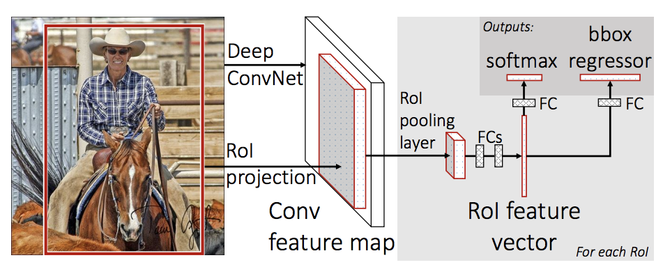
在本教程中，我們將使用 Mask R-CNN，它基於 Faster R-CNN。 Faster R-CNN 是一個可以預測圖像中潛在物件的邊界框和類別分數的模型。

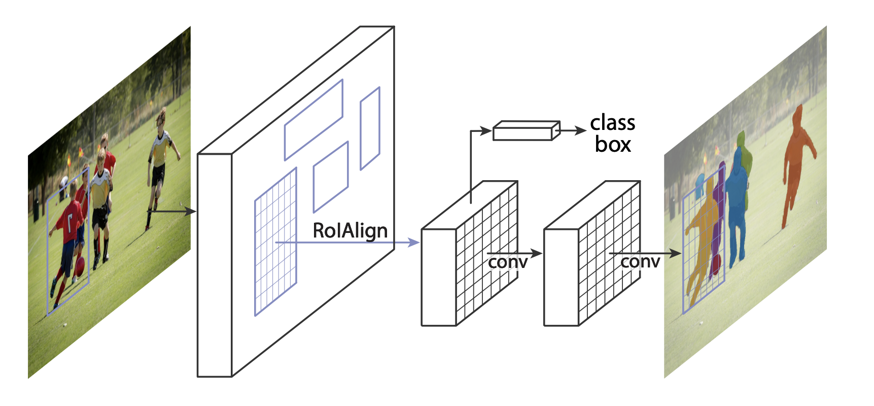
../_static/img/tv_tutorial/tv_image03.png

Mask R-CNN 在 Faster R-CNN 中添加了一個額外的分支，該分支還預測每個實例的分割遮罩。

../_static/img/tv_tutorial/tv_image04.png

在兩種常見的情況下，人們可能想要修改 TorchVision Model Zoo 中可用的模型之一。第一種是當我們想從預訓練模型開始，然後微調最後一層時。另一種情況是，當我們想用不同的 backbone 替換模型的 backbone 時（例如，為了更快的預測）。

讓我們看看如何在以下部分中執行其中一種或另一種。

1 - 從預訓練模型進行微調¶

假設你想從一個在 COCO 上預訓練的模型開始，並想針對你的特定類別進行微調。這是一種可行的方法

import torchvision
from torchvision.models.detection.faster_rcnn import FastRCNNPredictor

# load a model pre-trained on COCO
model = torchvision.models.detection.fasterrcnn_resnet50_fpn(weights="DEFAULT")

# replace the classifier with a new one, that has
# num_classes which is user-defined
num_classes = 2  # 1 class (person) + background
# get number of input features for the classifier
in_features = model.roi_heads.box_predictor.cls_score.in_features
# replace the pre-trained head with a new one
model.roi_heads.box_predictor = FastRCNNPredictor(in_features, num_classes)

Downloading: "https://download.pytorch.org/models/fasterrcnn_resnet50_fpn_coco-258fb6c6.pth" to /var/lib/ci-user/.cache/torch/hub/checkpoints/fasterrcnn_resnet50_fpn_coco-258fb6c6.pth

  0%|          | 0.00/160M [00:00<?, ?B/s]
 27%|##7       | 43.4M/160M [00:00<00:00, 454MB/s]
 55%|#####4    | 87.8M/160M [00:00<00:00, 461MB/s]
 83%|########2 | 132M/160M [00:00<00:00, 463MB/s]
100%|##########| 160M/160M [00:00<00:00, 462MB/s]

2 - 修改模型以添加不同的 backbone¶

import torchvision
from torchvision.models.detection import FasterRCNN
from torchvision.models.detection.rpn import AnchorGenerator

# load a pre-trained model for classification and return
# only the features
backbone = torchvision.models.mobilenet_v2(weights="DEFAULT").features
# ``FasterRCNN`` needs to know the number of
# output channels in a backbone. For mobilenet_v2, it's 1280
# so we need to add it here
backbone.out_channels = 1280

# let's make the RPN generate 5 x 3 anchors per spatial
# location, with 5 different sizes and 3 different aspect
# ratios. We have a Tuple[Tuple[int]] because each feature
# map could potentially have different sizes and
# aspect ratios
anchor_generator = AnchorGenerator(
    sizes=((32, 64, 128, 256, 512),),
    aspect_ratios=((0.5, 1.0, 2.0),)
)

# let's define what are the feature maps that we will
# use to perform the region of interest cropping, as well as
# the size of the crop after rescaling.
# if your backbone returns a Tensor, featmap_names is expected to
# be [0]. More generally, the backbone should return an
# ``OrderedDict[Tensor]``, and in ``featmap_names`` you can choose which
# feature maps to use.
roi_pooler = torchvision.ops.MultiScaleRoIAlign(
    featmap_names=['0'],
    output_size=7,
    sampling_ratio=2
)

# put the pieces together inside a Faster-RCNN model
model = FasterRCNN(
    backbone,
    num_classes=2,
    rpn_anchor_generator=anchor_generator,
    box_roi_pool=roi_pooler
)

Downloading: "https://download.pytorch.org/models/mobilenet_v2-7ebf99e0.pth" to /var/lib/ci-user/.cache/torch/hub/checkpoints/mobilenet_v2-7ebf99e0.pth

  0%|          | 0.00/13.6M [00:00<?, ?B/s]
100%|##########| 13.6M/13.6M [00:00<00:00, 421MB/s]

PennFudan 資料集的物件檢測和實例分割模型¶

在我們的例子中，我們想要從一個預訓練的模型進行微調，因為我們的資料集非常小，因此我們將遵循方法 1。

在這裡，我們也想要計算實例分割遮罩，因此我們將使用 Mask R-CNN

import torchvision
from torchvision.models.detection.faster_rcnn import FastRCNNPredictor
from torchvision.models.detection.mask_rcnn import MaskRCNNPredictor


def get_model_instance_segmentation(num_classes):
    # load an instance segmentation model pre-trained on COCO
    model = torchvision.models.detection.maskrcnn_resnet50_fpn(weights="DEFAULT")

    # get number of input features for the classifier
    in_features = model.roi_heads.box_predictor.cls_score.in_features
    # replace the pre-trained head with a new one
    model.roi_heads.box_predictor = FastRCNNPredictor(in_features, num_classes)

    # now get the number of input features for the mask classifier
    in_features_mask = model.roi_heads.mask_predictor.conv5_mask.in_channels
    hidden_layer = 256
    # and replace the mask predictor with a new one
    model.roi_heads.mask_predictor = MaskRCNNPredictor(
        in_features_mask,
        hidden_layer,
        num_classes
    )

    return model

就是這樣，這會讓 model 準備好在您的自定義數據集上進行訓練和評估。

將所有東西組合在一起¶

在 references/detection/ 中，我們有一些輔助函式來簡化檢測模型的訓練和評估。在這裡，我們將使用 references/detection/engine.py 和 references/detection/utils.py。只需將 references/detection 下的所有內容下載到您的資料夾中，然後在此處使用它們。如果您在 Linux 上有 wget，您可以使用以下命令下載它們

os.system("wget https://raw.githubusercontent.com/pytorch/vision/main/references/detection/engine.py")
os.system("wget https://raw.githubusercontent.com/pytorch/vision/main/references/detection/utils.py")
os.system("wget https://raw.githubusercontent.com/pytorch/vision/main/references/detection/coco_utils.py")
os.system("wget https://raw.githubusercontent.com/pytorch/vision/main/references/detection/coco_eval.py")
os.system("wget https://raw.githubusercontent.com/pytorch/vision/main/references/detection/transforms.py")

自 v0.15.0 以來，torchvision 提供了新的 Transforms API，可以輕鬆地為物件偵測和分割任務編寫數據增強流程。

讓我們編寫一些用於數據增強/轉換的輔助函式

from torchvision.transforms import v2 as T


def get_transform(train):
    transforms = []
    if train:
        transforms.append(T.RandomHorizontalFlip(0.5))
    transforms.append(T.ToDtype(torch.float, scale=True))
    transforms.append(T.ToPureTensor())
    return T.Compose(transforms)

測試 `forward()` 方法 (選用)¶

在迭代數據集之前，最好先了解模型在樣本數據上的訓練和推論期間期望的輸入是什麼。

import utils

model = torchvision.models.detection.fasterrcnn_resnet50_fpn(weights="DEFAULT")
dataset = PennFudanDataset('data/PennFudanPed', get_transform(train=True))
data_loader = torch.utils.data.DataLoader(
    dataset,
    batch_size=2,
    shuffle=True,
    collate_fn=utils.collate_fn
)

# For Training
images, targets = next(iter(data_loader))
images = list(image for image in images)
targets = [{k: v for k, v in t.items()} for t in targets]
output = model(images, targets)  # Returns losses and detections
print(output)

# For inference
model.eval()
x = [torch.rand(3, 300, 400), torch.rand(3, 500, 400)]
predictions = model(x)  # Returns predictions
print(predictions[0])

{'loss_classifier': tensor(0.0808, grad_fn=<NllLossBackward0>), 'loss_box_reg': tensor(0.0284, grad_fn=<DivBackward0>), 'loss_objectness': tensor(0.0186, grad_fn=<BinaryCrossEntropyWithLogitsBackward0>), 'loss_rpn_box_reg': tensor(0.0034, grad_fn=<DivBackward0>)}
{'boxes': tensor([], size=(0, 4), grad_fn=<StackBackward0>), 'labels': tensor([], dtype=torch.int64), 'scores': tensor([], grad_fn=<IndexBackward0>)}

現在讓我們編寫執行訓練和驗證的主函式

from engine import train_one_epoch, evaluate

# train on the GPU or on the CPU, if a GPU is not available
device = torch.device('cuda') if torch.cuda.is_available() else torch.device('cpu')

# our dataset has two classes only - background and person
num_classes = 2
# use our dataset and defined transformations
dataset = PennFudanDataset('data/PennFudanPed', get_transform(train=True))
dataset_test = PennFudanDataset('data/PennFudanPed', get_transform(train=False))

# split the dataset in train and test set
indices = torch.randperm(len(dataset)).tolist()
dataset = torch.utils.data.Subset(dataset, indices[:-50])
dataset_test = torch.utils.data.Subset(dataset_test, indices[-50:])

# define training and validation data loaders
data_loader = torch.utils.data.DataLoader(
    dataset,
    batch_size=2,
    shuffle=True,
    collate_fn=utils.collate_fn
)

data_loader_test = torch.utils.data.DataLoader(
    dataset_test,
    batch_size=1,
    shuffle=False,
    collate_fn=utils.collate_fn
)

# get the model using our helper function
model = get_model_instance_segmentation(num_classes)

# move model to the right device
model.to(device)

# construct an optimizer
params = [p for p in model.parameters() if p.requires_grad]
optimizer = torch.optim.SGD(
    params,
    lr=0.005,
    momentum=0.9,
    weight_decay=0.0005
)

# and a learning rate scheduler
lr_scheduler = torch.optim.lr_scheduler.StepLR(
    optimizer,
    step_size=3,
    gamma=0.1
)

# let's train it just for 2 epochs
num_epochs = 2

for epoch in range(num_epochs):
    # train for one epoch, printing every 10 iterations
    train_one_epoch(model, optimizer, data_loader, device, epoch, print_freq=10)
    # update the learning rate
    lr_scheduler.step()
    # evaluate on the test dataset
    evaluate(model, data_loader_test, device=device)

print("That's it!")

Downloading: "https://download.pytorch.org/models/maskrcnn_resnet50_fpn_coco-bf2d0c1e.pth" to /var/lib/ci-user/.cache/torch/hub/checkpoints/maskrcnn_resnet50_fpn_coco-bf2d0c1e.pth

  0%|          | 0.00/170M [00:00<?, ?B/s]
  9%|8         | 14.5M/170M [00:00<00:01, 151MB/s]
 17%|#7        | 29.0M/170M [00:00<00:01, 142MB/s]
 43%|####2     | 72.4M/170M [00:00<00:00, 280MB/s]
 69%|######8   | 116M/170M [00:00<00:00, 350MB/s]
 94%|#########4| 160M/170M [00:00<00:00, 389MB/s]
100%|##########| 170M/170M [00:00<00:00, 333MB/s]
/var/lib/workspace/intermediate_source/engine.py:30: FutureWarning:

`torch.cuda.amp.autocast(args...)` is deprecated. Please use `torch.amp.autocast('cuda', args...)` instead.

Epoch: [0]  [ 0/60]  eta: 0:00:23  lr: 0.000090  loss: 4.9024 (4.9024)  loss_classifier: 0.4325 (0.4325)  loss_box_reg: 0.1060 (0.1060)  loss_mask: 4.3588 (4.3588)  loss_objectness: 0.0028 (0.0028)  loss_rpn_box_reg: 0.0023 (0.0023)  time: 0.3936  data: 0.0141  max mem: 2430
Epoch: [0]  [10/60]  eta: 0:00:11  lr: 0.000936  loss: 1.7766 (2.7700)  loss_classifier: 0.4105 (0.3557)  loss_box_reg: 0.3052 (0.2546)  loss_mask: 0.9490 (2.1314)  loss_objectness: 0.0219 (0.0214)  loss_rpn_box_reg: 0.0056 (0.0069)  time: 0.2282  data: 0.0157  max mem: 2602
Epoch: [0]  [20/60]  eta: 0:00:08  lr: 0.001783  loss: 0.8104 (1.7885)  loss_classifier: 0.2146 (0.2679)  loss_box_reg: 0.2065 (0.2333)  loss_mask: 0.3977 (1.2590)  loss_objectness: 0.0134 (0.0202)  loss_rpn_box_reg: 0.0076 (0.0080)  time: 0.2082  data: 0.0159  max mem: 2624
Epoch: [0]  [30/60]  eta: 0:00:06  lr: 0.002629  loss: 0.6767 (1.4244)  loss_classifier: 0.1406 (0.2261)  loss_box_reg: 0.2294 (0.2435)  loss_mask: 0.2592 (0.9277)  loss_objectness: 0.0120 (0.0173)  loss_rpn_box_reg: 0.0101 (0.0098)  time: 0.2122  data: 0.0169  max mem: 2771
Epoch: [0]  [40/60]  eta: 0:00:04  lr: 0.003476  loss: 0.5520 (1.2053)  loss_classifier: 0.0892 (0.1909)  loss_box_reg: 0.2434 (0.2359)  loss_mask: 0.2266 (0.7542)  loss_objectness: 0.0069 (0.0145)  loss_rpn_box_reg: 0.0118 (0.0098)  time: 0.2105  data: 0.0169  max mem: 2771
Epoch: [0]  [50/60]  eta: 0:00:02  lr: 0.004323  loss: 0.3561 (1.0396)  loss_classifier: 0.0567 (0.1626)  loss_box_reg: 0.1485 (0.2173)  loss_mask: 0.1633 (0.6383)  loss_objectness: 0.0021 (0.0121)  loss_rpn_box_reg: 0.0072 (0.0093)  time: 0.2051  data: 0.0158  max mem: 2771
Epoch: [0]  [59/60]  eta: 0:00:00  lr: 0.005000  loss: 0.3503 (0.9406)  loss_classifier: 0.0384 (0.1447)  loss_box_reg: 0.1258 (0.2049)  loss_mask: 0.1614 (0.5713)  loss_objectness: 0.0011 (0.0107)  loss_rpn_box_reg: 0.0064 (0.0089)  time: 0.2035  data: 0.0150  max mem: 2771
Epoch: [0] Total time: 0:00:12 (0.2108 s / it)
creating index...
index created!
Test:  [ 0/50]  eta: 0:00:04  model_time: 0.0796 (0.0796)  evaluator_time: 0.0073 (0.0073)  time: 0.0995  data: 0.0122  max mem: 2771
Test:  [49/50]  eta: 0:00:00  model_time: 0.0422 (0.0569)  evaluator_time: 0.0049 (0.0068)  time: 0.0644  data: 0.0096  max mem: 2771
Test: Total time: 0:00:03 (0.0748 s / it)
Averaged stats: model_time: 0.0422 (0.0569)  evaluator_time: 0.0049 (0.0068)
Accumulating evaluation results...
DONE (t=0.01s).
Accumulating evaluation results...
DONE (t=0.01s).
IoU metric: bbox
 Average Precision  (AP) @[ IoU=0.50:0.95 | area=   all | maxDets=100 ] = 0.634
 Average Precision  (AP) @[ IoU=0.50      | area=   all | maxDets=100 ] = 0.984
 Average Precision  (AP) @[ IoU=0.75      | area=   all | maxDets=100 ] = 0.868
 Average Precision  (AP) @[ IoU=0.50:0.95 | area= small | maxDets=100 ] = 0.288
 Average Precision  (AP) @[ IoU=0.50:0.95 | area=medium | maxDets=100 ] = 0.599
 Average Precision  (AP) @[ IoU=0.50:0.95 | area= large | maxDets=100 ] = 0.644
 Average Recall     (AR) @[ IoU=0.50:0.95 | area=   all | maxDets=  1 ] = 0.279
 Average Recall     (AR) @[ IoU=0.50:0.95 | area=   all | maxDets= 10 ] = 0.689
 Average Recall     (AR) @[ IoU=0.50:0.95 | area=   all | maxDets=100 ] = 0.689
 Average Recall     (AR) @[ IoU=0.50:0.95 | area= small | maxDets=100 ] = 0.367
 Average Recall     (AR) @[ IoU=0.50:0.95 | area=medium | maxDets=100 ] = 0.683
 Average Recall     (AR) @[ IoU=0.50:0.95 | area= large | maxDets=100 ] = 0.698
IoU metric: segm
 Average Precision  (AP) @[ IoU=0.50:0.95 | area=   all | maxDets=100 ] = 0.668
 Average Precision  (AP) @[ IoU=0.50      | area=   all | maxDets=100 ] = 0.974
 Average Precision  (AP) @[ IoU=0.75      | area=   all | maxDets=100 ] = 0.782
 Average Precision  (AP) @[ IoU=0.50:0.95 | area= small | maxDets=100 ] = 0.394
 Average Precision  (AP) @[ IoU=0.50:0.95 | area=medium | maxDets=100 ] = 0.501
 Average Precision  (AP) @[ IoU=0.50:0.95 | area= large | maxDets=100 ] = 0.682
 Average Recall     (AR) @[ IoU=0.50:0.95 | area=   all | maxDets=  1 ] = 0.292
 Average Recall     (AR) @[ IoU=0.50:0.95 | area=   all | maxDets= 10 ] = 0.724
 Average Recall     (AR) @[ IoU=0.50:0.95 | area=   all | maxDets=100 ] = 0.725
 Average Recall     (AR) @[ IoU=0.50:0.95 | area= small | maxDets=100 ] = 0.633
 Average Recall     (AR) @[ IoU=0.50:0.95 | area=medium | maxDets=100 ] = 0.683
 Average Recall     (AR) @[ IoU=0.50:0.95 | area= large | maxDets=100 ] = 0.732
Epoch: [1]  [ 0/60]  eta: 0:00:11  lr: 0.005000  loss: 0.2638 (0.2638)  loss_classifier: 0.0195 (0.0195)  loss_box_reg: 0.0624 (0.0624)  loss_mask: 0.1786 (0.1786)  loss_objectness: 0.0001 (0.0001)  loss_rpn_box_reg: 0.0032 (0.0032)  time: 0.1853  data: 0.0139  max mem: 2771
Epoch: [1]  [10/60]  eta: 0:00:10  lr: 0.005000  loss: 0.3414 (0.3752)  loss_classifier: 0.0520 (0.0535)  loss_box_reg: 0.1229 (0.1440)  loss_mask: 0.1642 (0.1661)  loss_objectness: 0.0029 (0.0034)  loss_rpn_box_reg: 0.0082 (0.0082)  time: 0.2082  data: 0.0162  max mem: 2771
Epoch: [1]  [20/60]  eta: 0:00:08  lr: 0.005000  loss: 0.3414 (0.3467)  loss_classifier: 0.0380 (0.0449)  loss_box_reg: 0.1204 (0.1173)  loss_mask: 0.1676 (0.1750)  loss_objectness: 0.0016 (0.0024)  loss_rpn_box_reg: 0.0069 (0.0071)  time: 0.2039  data: 0.0152  max mem: 2771
Epoch: [1]  [30/60]  eta: 0:00:06  lr: 0.005000  loss: 0.3095 (0.3290)  loss_classifier: 0.0367 (0.0450)  loss_box_reg: 0.0884 (0.1121)  loss_mask: 0.1445 (0.1630)  loss_objectness: 0.0009 (0.0022)  loss_rpn_box_reg: 0.0044 (0.0068)  time: 0.2044  data: 0.0152  max mem: 2771
Epoch: [1]  [40/60]  eta: 0:00:04  lr: 0.005000  loss: 0.2793 (0.3223)  loss_classifier: 0.0429 (0.0439)  loss_box_reg: 0.0884 (0.1060)  loss_mask: 0.1444 (0.1633)  loss_objectness: 0.0011 (0.0021)  loss_rpn_box_reg: 0.0052 (0.0070)  time: 0.2055  data: 0.0159  max mem: 2771
Epoch: [1]  [50/60]  eta: 0:00:02  lr: 0.005000  loss: 0.2681 (0.3110)  loss_classifier: 0.0314 (0.0420)  loss_box_reg: 0.0583 (0.0992)  loss_mask: 0.1519 (0.1614)  loss_objectness: 0.0009 (0.0019)  loss_rpn_box_reg: 0.0045 (0.0065)  time: 0.2030  data: 0.0149  max mem: 2771
Epoch: [1]  [59/60]  eta: 0:00:00  lr: 0.005000  loss: 0.2230 (0.2965)  loss_classifier: 0.0314 (0.0406)  loss_box_reg: 0.0499 (0.0927)  loss_mask: 0.1296 (0.1551)  loss_objectness: 0.0005 (0.0018)  loss_rpn_box_reg: 0.0031 (0.0062)  time: 0.2051  data: 0.0155  max mem: 2771
Epoch: [1] Total time: 0:00:12 (0.2048 s / it)
creating index...
index created!
Test:  [ 0/50]  eta: 0:00:02  model_time: 0.0442 (0.0442)  evaluator_time: 0.0032 (0.0032)  time: 0.0600  data: 0.0121  max mem: 2771
Test:  [49/50]  eta: 0:00:00  model_time: 0.0398 (0.0409)  evaluator_time: 0.0028 (0.0040)  time: 0.0544  data: 0.0096  max mem: 2771
Test: Total time: 0:00:02 (0.0559 s / it)
Averaged stats: model_time: 0.0398 (0.0409)  evaluator_time: 0.0028 (0.0040)
Accumulating evaluation results...
DONE (t=0.01s).
Accumulating evaluation results...
DONE (t=0.01s).
IoU metric: bbox
 Average Precision  (AP) @[ IoU=0.50:0.95 | area=   all | maxDets=100 ] = 0.751
 Average Precision  (AP) @[ IoU=0.50      | area=   all | maxDets=100 ] = 0.986
 Average Precision  (AP) @[ IoU=0.75      | area=   all | maxDets=100 ] = 0.929
 Average Precision  (AP) @[ IoU=0.50:0.95 | area= small | maxDets=100 ] = 0.465
 Average Precision  (AP) @[ IoU=0.50:0.95 | area=medium | maxDets=100 ] = 0.684
 Average Precision  (AP) @[ IoU=0.50:0.95 | area= large | maxDets=100 ] = 0.765
 Average Recall     (AR) @[ IoU=0.50:0.95 | area=   all | maxDets=  1 ] = 0.320
 Average Recall     (AR) @[ IoU=0.50:0.95 | area=   all | maxDets= 10 ] = 0.798
 Average Recall     (AR) @[ IoU=0.50:0.95 | area=   all | maxDets=100 ] = 0.798
 Average Recall     (AR) @[ IoU=0.50:0.95 | area= small | maxDets=100 ] = 0.467
 Average Recall     (AR) @[ IoU=0.50:0.95 | area=medium | maxDets=100 ] = 0.767
 Average Recall     (AR) @[ IoU=0.50:0.95 | area= large | maxDets=100 ] = 0.811
IoU metric: segm
 Average Precision  (AP) @[ IoU=0.50:0.95 | area=   all | maxDets=100 ] = 0.725
 Average Precision  (AP) @[ IoU=0.50      | area=   all | maxDets=100 ] = 0.972
 Average Precision  (AP) @[ IoU=0.75      | area=   all | maxDets=100 ] = 0.891
 Average Precision  (AP) @[ IoU=0.50:0.95 | area= small | maxDets=100 ] = 0.394
 Average Precision  (AP) @[ IoU=0.50:0.95 | area=medium | maxDets=100 ] = 0.577
 Average Precision  (AP) @[ IoU=0.50:0.95 | area= large | maxDets=100 ] = 0.742
 Average Recall     (AR) @[ IoU=0.50:0.95 | area=   all | maxDets=  1 ] = 0.313
 Average Recall     (AR) @[ IoU=0.50:0.95 | area=   all | maxDets= 10 ] = 0.768
 Average Recall     (AR) @[ IoU=0.50:0.95 | area=   all | maxDets=100 ] = 0.768
 Average Recall     (AR) @[ IoU=0.50:0.95 | area= small | maxDets=100 ] = 0.533
 Average Recall     (AR) @[ IoU=0.50:0.95 | area=medium | maxDets=100 ] = 0.708
 Average Recall     (AR) @[ IoU=0.50:0.95 | area= large | maxDets=100 ] = 0.780
That's it!

因此，經過一個 epoch 的訓練後，我們獲得了 COCO 風格的 mAP > 50，以及 mask mAP 為 65。

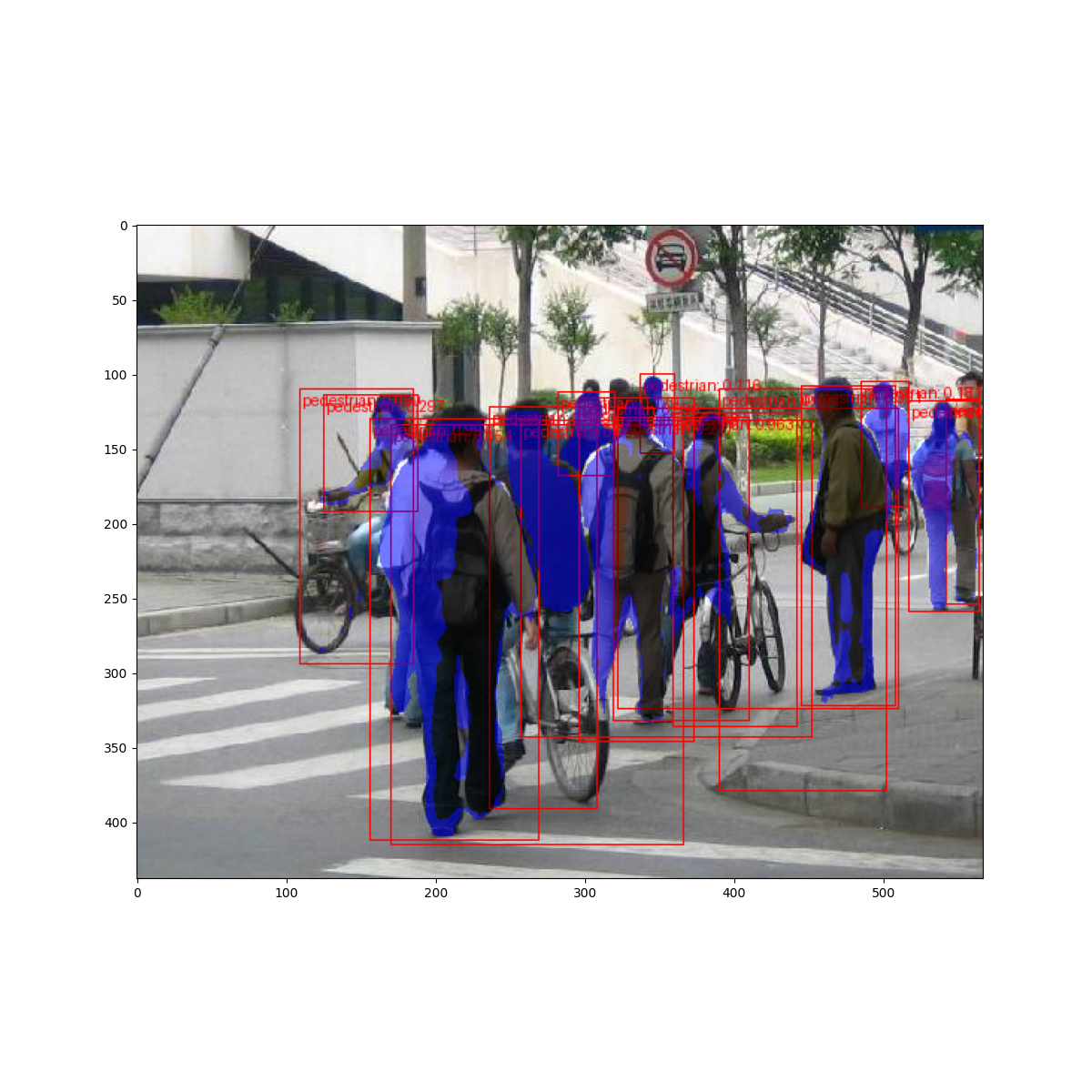
但是預測結果看起來如何？讓我們在數據集中取一張圖像並進行驗證

import matplotlib.pyplot as plt

from torchvision.utils import draw_bounding_boxes, draw_segmentation_masks


image = read_image("data/PennFudanPed/PNGImages/FudanPed00046.png")
eval_transform = get_transform(train=False)

model.eval()
with torch.no_grad():
    x = eval_transform(image)
    # convert RGBA -> RGB and move to device
    x = x[:3, ...].to(device)
    predictions = model([x, ])
    pred = predictions[0]


image = (255.0 * (image - image.min()) / (image.max() - image.min())).to(torch.uint8)
image = image[:3, ...]
pred_labels = [f"pedestrian: {score:.3f}" for label, score in zip(pred["labels"], pred["scores"])]
pred_boxes = pred["boxes"].long()
output_image = draw_bounding_boxes(image, pred_boxes, pred_labels, colors="red")

masks = (pred["masks"] > 0.7).squeeze(1)
output_image = draw_segmentation_masks(output_image, masks, alpha=0.5, colors="blue")


plt.figure(figsize=(12, 12))
plt.imshow(output_image.permute(1, 2, 0))

<matplotlib.image.AxesImage object at 0x7f3691de7d00>

結果看起來不錯！

總結¶

在本教學中，您學習了如何為自定義數據集上的物件偵測模型建立自己的訓練流程。為此，您編寫了一個 torch.utils.data.Dataset 類，該類別會傳回圖像和 ground truth box 和分割遮罩。您還利用了在 COCO train2017 上預先訓練的 Mask R-CNN 模型，以便在此新數據集上執行遷移學習。

如需更完整的範例，包括多機器/多 GPU 訓練，請查看 torchvision 儲存庫中的 references/detection/train.py。

腳本總執行時間： ( 0 分鐘 45.484 秒)

由 Sphinx-Gallery 產生圖庫