


使用 PyTorch 和 TIAToolbox 進行全玻片影像分類
建立於:2023 年 12 月 19 日 | 最後更新:2024 年 8 月 27 日 | 最後驗證:2024 年 11 月 05 日
提示
為了充分利用本教學,我們建議使用此Colab 版本。 這將允許您嘗試以下提供的資訊。
簡介
在本教學中,我們將展示如何借助 TIAToolbox,使用 PyTorch 深度學習模型對全玻片影像 (WSI) 進行分類。 WSI 是透過手術或活組織切片取得的人體組織樣本影像,並使用專用掃描器進行掃描。 病理學家和計算病理學研究人員使用它們來在顯微鏡下研究癌症等疾病,以便例如了解腫瘤生長並幫助改善患者的治療。
使 WSI 難以處理的原因在於它們的巨大尺寸。 例如,典型的玻片影像具有大約 100,000x100,000 像素的數量級,其中每個像素可以對應於玻片上大約 0.25x0.25 微米。 這在載入和處理此類影像時帶來了挑戰,更不用說單項研究中數百甚至數千個 WSI(較大的研究產生更好的結果)!
傳統的影像處理管線不適用於 WSI 處理,因此我們需要更好的工具。 這就是 TIAToolbox 可以提供幫助的地方,因為它帶來了一組有用的工具,可以快速且計算效率高地匯入和處理組織玻片。 通常,WSI 以金字塔結構儲存,同一影像在各種放大倍率下有多個副本,並針對視覺化進行了最佳化。 金字塔的第 0 層(或底層)包含最高放大倍率或縮放級別的影像,而金字塔中較高的層具有基本影像的較低解析度副本。 金字塔結構如下所示。
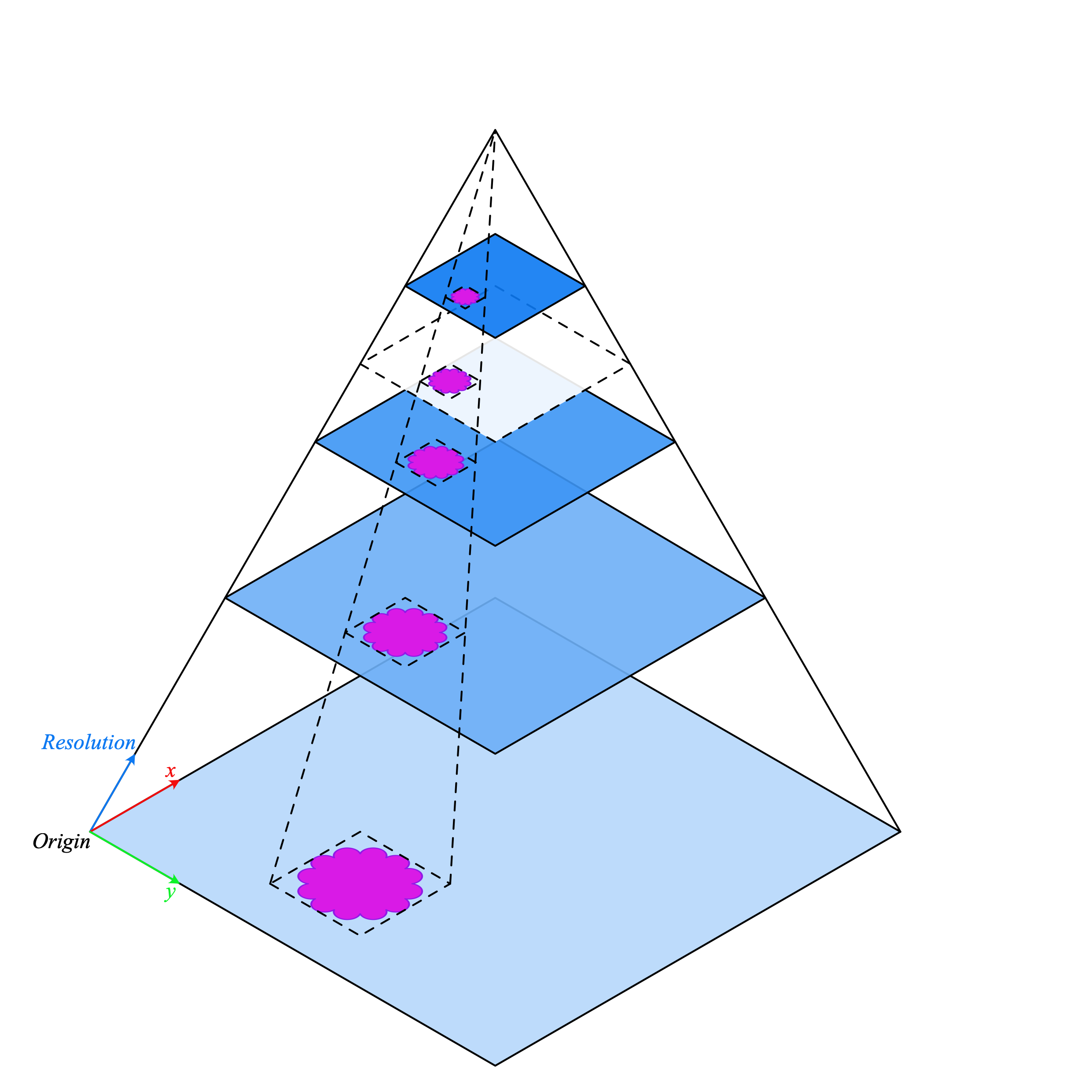 WSI 金字塔堆疊 (來源)
TIAToolbox 允許我們自動化常見的下游分析任務,例如組織分類。 在本教學中,我們將展示如何:1. 使用 TIAToolbox 載入 WSI 影像; 以及 2. 使用不同的 PyTorch 模型在圖塊層級對玻片進行分類。 在本教學中,我們將提供使用 TorchVision ResNet18 模型和自訂 HistoEncoder <https://github.com/jopo666/HistoEncoder>`__ 模型的範例。
讓我們開始吧!
設定環境
若要執行本教學中提供的範例,需要以下套件作為先決條件。
OpenJpeg
OpenSlide
Pixman
TIAToolbox
HistoEncoder(用於自訂模型範例)
請在您的終端機中執行以下命令以安裝這些套件
apt-get -y -qq install libopenjp2-7-dev libopenjp2-tools openslide-tools libpixman-1-dev pip install -q ‘tiatoolbox<1.5’ histoencoder && echo “Installation is done.”
或者,您可以執行 brew install openjpeg openslide 以在 MacOS 上安裝先決條件套件,而不是 apt-get。 有關安裝的更多資訊可以在這裡找到。
執行前清理
為了確保適當的清理(例如在異常終止時),本次執行中下載或建立的所有檔案都會儲存在單一目錄 global_save_dir 中,我們將其設定為“./tmp/”。為了簡化維護,目錄名稱只會出現在這個地方,以便在需要時可以輕鬆更改。
warnings.filterwarnings("ignore")
global_save_dir = Path("./tmp/")


def rmdir(dir_path: str | Path) -> None:
    """Helper function to delete directory."""
    if Path(dir_path).is_dir():
        shutil.rmtree(dir_path)
        logger.info("Removing directory %s", dir_path)


rmdir(global_save_dir)  # remove  directory if it exists from previous runs
global_save_dir.mkdir()
logger.info("Creating new directory %s", global_save_dir)
下載資料
對於我們的範例資料,我們將使用一張完整的切片影像,以及來自 Kather 100k 資料集驗證子集的圖像塊。
wsi_path = global_save_dir / "sample_wsi.svs"
patches_path = global_save_dir / "kather100k-validation-sample.zip"
weights_path = global_save_dir / "resnet18-kather100k.pth"

logger.info("Download has started. Please wait...")

# Downloading and unzip a sample whole-slide image
download_data(
    "https://tiatoolbox.dcs.warwick.ac.uk/sample_wsis/TCGA-3L-AA1B-01Z-00-DX1.8923A151-A690-40B7-9E5A-FCBEDFC2394F.svs",
    wsi_path,
)

# Download and unzip a sample of the validation set used to train the Kather 100K dataset
download_data(
    "https://tiatoolbox.dcs.warwick.ac.uk/datasets/kather100k-validation-sample.zip",
    patches_path,
)
with ZipFile(patches_path, "r") as zipfile:
    zipfile.extractall(path=global_save_dir)

# Download pretrained model weights for WSI classification using ResNet18 architecture
download_data(
    "https://tiatoolbox.dcs.warwick.ac.uk/models/pc/resnet18-kather100k.pth",
    weights_path,
)

logger.info("Download is complete.")
讀取資料
我們建立一個圖像塊列表和一個對應標籤列表。例如,label_list 中的第一個標籤將指示 patch_list 中第一個圖像塊的類別。
# Read the patch data and create a list of patches and a list of corresponding labels
dataset_path = global_save_dir / "kather100k-validation-sample"
# Set the path to the dataset
image_ext = ".tif" # file extension of each image
# Obtain the mapping between the label ID and the class name
label_dict = {
"BACK": 0, # Background (empty glass region)
"NORM": 1, # Normal colon mucosa
"DEB": 2, # Debris
"TUM": 3, # Colorectal adenocarcinoma epithelium
"ADI": 4, # Adipose
"MUC": 5, # Mucus
"MUS": 6, # Smooth muscle
"STR": 7, # Cancer-associated stroma
"LYM": 8, # Lymphocytes
}
class_names = list(label_dict.keys())
class_labels = list(label_dict.values())
# Generate a list of patches and generate the label from the filename
patch_list = []
label_list = []
for class_name, label in label_dict.items():
dataset_class_path = dataset_path / class_name
patch_list_single_class = grab_files_from_dir(
dataset_class_path,
file_types="*" + image_ext,
)
patch_list.extend(patch_list_single_class)
label_list.extend([label] * len(patch_list_single_class))
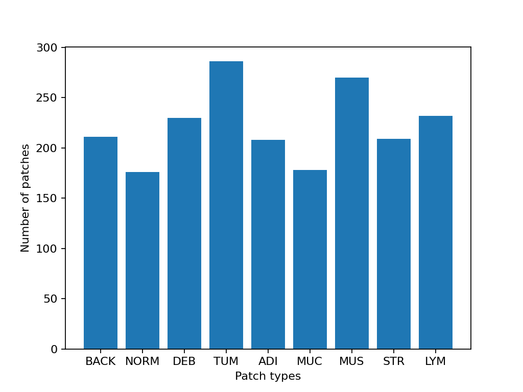
# Show some dataset statistics
plt.bar(class_names, [label_list.count(label) for label in class_labels])
plt.xlabel("Patch types")
plt.ylabel("Number of patches")
# Count the number of examples per class
for class_name, label in label_dict.items():
logger.info(
"Class ID: %d -- Class Name: %s -- Number of images: %d",
label,
class_name,
label_list.count(label),
)
# Overall dataset statistics
logger.info("Total number of patches: %d", (len(patch_list)))
|2023-11-14|13:15:59.299| [INFO] Class ID: 0 -- Class Name: BACK -- Number of images: 211
|2023-11-14|13:15:59.299| [INFO] Class ID: 1 -- Class Name: NORM -- Number of images: 176
|2023-11-14|13:15:59.299| [INFO] Class ID: 2 -- Class Name: DEB -- Number of images: 230
|2023-11-14|13:15:59.299| [INFO] Class ID: 3 -- Class Name: TUM -- Number of images: 286
|2023-11-14|13:15:59.299| [INFO] Class ID: 4 -- Class Name: ADI -- Number of images: 208
|2023-11-14|13:15:59.299| [INFO] Class ID: 5 -- Class Name: MUC -- Number of images: 178
|2023-11-14|13:15:59.299| [INFO] Class ID: 6 -- Class Name: MUS -- Number of images: 270
|2023-11-14|13:15:59.299| [INFO] Class ID: 7 -- Class Name: STR -- Number of images: 209
|2023-11-14|13:15:59.299| [INFO] Class ID: 8 -- Class Name: LYM -- Number of images: 232
|2023-11-14|13:15:59.299| [INFO] Total number of patches: 2000
如您所見,對於此圖像塊資料集,我們有 9 個類別/標籤,ID 為 0-8,以及相關的類別名稱,用於描述圖像塊中的主要組織類型。
BACK ⟶ 背景(空的玻璃區域)
LYM ⟶ 淋巴細胞
NORM ⟶ 正常結腸黏膜
DEB ⟶ 碎片
MUS ⟶ 平滑肌
STR ⟶ 癌症相關基質
ADI ⟶ 脂肪
MUC ⟶ 黏液
TUM ⟶ 結直腸腺癌上皮
分類圖像塊
我們示範如何首先使用 patch 模式,然後使用 wsi 模式,取得數位切片中每個圖像塊的預測。
定義 PatchPredictor 模型
PatchPredictor 類別執行一個以 PyTorch 撰寫的基於 CNN 的分類器。
model可以是任何經過訓練的 PyTorch 模型,但它應該遵循tiatoolbox.models.abc.ModelABC(docs) <https://tia-toolbox.readthedocs.io/en/latest/_autosummary/tiatoolbox.models.models_abc.ModelABC.html>`__ 類別結構。 有關此事的更多資訊,請參閱 我們關於進階模型技術的範例筆記本。 為了載入自訂模型,您需要編寫一個小的預處理函數,例如preproc_func(img),以確保輸入張量對於載入的網路具有正確的格式。或者,您可以傳遞
pretrained_model作為字串引數。 這指定了執行預測的 CNN 模型,它必須是 此處 列出的模型之一。 命令看起來像這樣:predictor = PatchPredictor(pretrained_model='resnet18-kather100k', pretrained_weights=weights_path, batch_size=32)。pretrained_weights: 當使用pretrained_model時,預設情況下也會下載相應的預訓練權重。 您可以使用pretrained_weight引數,以您自己的權重集覆蓋預設值。batch_size:每次饋入模型的圖像數量。 此參數的較高值需要較大的(GPU)記憶體容量。
# Importing a pretrained PyTorch model from TIAToolbox
predictor = PatchPredictor(pretrained_model='resnet18-kather100k', batch_size=32)

# Users can load any PyTorch model architecture instead using the following script
model = vanilla.CNNModel(backbone="resnet18", num_classes=9) # Importing model from torchvision.models.resnet18
model.load_state_dict(torch.load(weights_path, map_location="cpu", weights_only=True), strict=True)
def preproc_func(img):
    img = PIL.Image.fromarray(img)
    img = transforms.ToTensor()(img)
    return img.permute(1, 2, 0)
model.preproc_func = preproc_func
predictor = PatchPredictor(model=model, batch_size=32)
預測圖像塊標籤
我們建立一個預測器物件,然後使用 patch 模式呼叫 predict 方法。 然後,我們計算分類準確度和混淆矩陣。
with suppress_console_output():
    output = predictor.predict(imgs=patch_list, mode="patch", on_gpu=ON_GPU)

acc = accuracy_score(label_list, output["predictions"])
logger.info("Classification accuracy: %f", acc)

# Creating and visualizing the confusion matrix for patch classification results
conf = confusion_matrix(label_list, output["predictions"], normalize="true")
df_cm = pd.DataFrame(conf, index=class_names, columns=class_names)
df_cm
|2023-11-14|13:16:03.215| [INFO] Classification accuracy: 0.993000
預測整張切片的圖像塊標籤
我們現在介紹 IOPatchPredictorConfig,這是一個用於指定模型預測引擎的圖像讀取和預測寫入配置的類別。 這是必須的,以便告知分類器應讀取 WSI 金字塔的哪個層級、處理資料並產生輸出。
IOPatchPredictorConfig 的參數定義如下
input_resolutions:一個列表,以字典的形式指定每個輸入的分辨率。 列表元素必須與目標model.forward()中的順序相同。 如果您的模型只接受一個輸入,您只需要放置一個字典,指定'units'和'resolution'。 請注意,TIAToolbox 支援具有多個輸入的模型。 有關單位和分辨率的更多資訊,請參閱 TIAToolbox 文件。patch_input_shape:最大輸入的形狀,格式為 (高度, 寬度)。stride_shape:在圖像塊提取過程中,兩個連續圖像塊之間的步幅(步驟)大小。 如果使用者將stride_shape設定為等於patch_input_shape,則將提取和處理圖像塊,而不會有任何重疊。
wsi_ioconfig = IOPatchPredictorConfig(
    input_resolutions=[{"units": "mpp", "resolution": 0.5}],
    patch_input_shape=[224, 224],
    stride_shape=[224, 224],
)
predict 方法將 CNN 應用於輸入圖像塊並取得結果。 以下是引數及其說明
mode:要處理的輸入類型。 根據您的應用程式,從patch、tile或wsi中選擇。imgs:輸入列表,應該是輸入圖塊或 WSI 的路徑列表。return_probabilities:設定為 True 以取得每個類別的機率,以及輸入圖像塊的預測標籤。 如果您希望合併預測以產生tile或wsi模式的預測地圖,您可以設定return_probabilities=True。ioconfig:使用IOPatchPredictorConfig類別設定 IO 配置資訊。resolution和unit(如下未顯示):這些參數指定了 WSI 層級的解析度或每像素微米數,我們計劃從這些層級提取圖塊,並且可以用來替代ioconfig。 這裡我們將 WSI 層級指定為'baseline',它等同於層級 0。 一般來說,這是解析度最高的層級。 在這個特定的例子中,影像只有一個層級。 更多資訊可以在文檔中找到。masks:一個路徑列表,對應於imgs列表中 WSI 的遮罩。 這些遮罩指定了原始 WSI 中我們想要提取圖塊的區域。 如果特定 WSI 的遮罩被指定為None,那麼該 WSI 的所有圖塊(甚至包括背景區域)的標籤都會被預測。 這可能會導致不必要的計算。merge_predictions:如果需要生成圖塊分類結果的 2D 地圖,您可以將此參數設定為True。 然而,對於大型 WSI,這將需要大量的可用記憶體。 另一種(預設)解決方案是將merge_predictions=False設定為 false,然後使用merge_predictions函數生成 2D 預測地圖,您將在稍後看到。
由於我們正在使用大型 WSI,圖塊提取和預測過程可能需要一些時間(如果您可以使用 Cuda enabled GPU 和 PyTorch+Cuda,請務必設定 ON_GPU=True)。
with suppress_console_output():
    wsi_output = predictor.predict(
        imgs=[wsi_path],
        masks=None,
        mode="wsi",
        merge_predictions=False,
        ioconfig=wsi_ioconfig,
        return_probabilities=True,
        save_dir=global_save_dir / "wsi_predictions",
        on_gpu=ON_GPU,
    )
我們透過可視化 wsi_output 來了解預測模型在我們的 whole-slide 影像上的工作方式。 我們首先需要合併圖塊預測輸出,然後將它們作為原始影像上的疊加層可視化。 和以前一樣,merge_predictions 方法用於合併圖塊預測。 這裡,我們設定參數 resolution=1.25, units='power',以 1.25 倍放大倍率生成預測地圖。 如果您想要更高/更低解析度(更大/更小)的預測地圖,您需要相應地更改這些參數。 當預測合併後,使用 overlay_patch_prediction 函數將預測地圖疊加在 WSI 縮圖上,該縮圖應以用於預測合併的解析度提取。
overview_resolution = (
    4  # the resolution in which we desire to merge and visualize the patch predictions
)
# the unit of the `resolution` parameter. Can be "power", "level", "mpp", or "baseline"
overview_unit = "mpp"
wsi = WSIReader.open(wsi_path)
wsi_overview = wsi.slide_thumbnail(resolution=overview_resolution, units=overview_unit)
plt.figure(), plt.imshow(wsi_overview)
plt.axis("off")
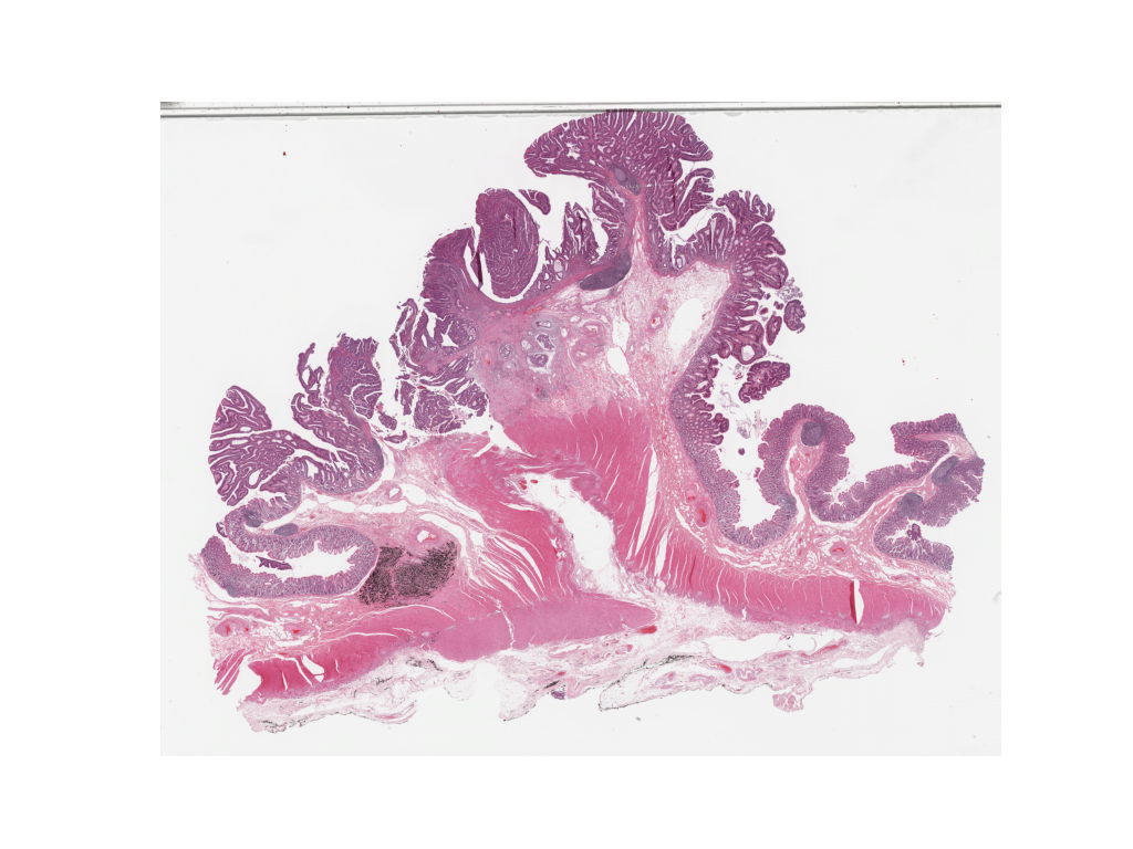
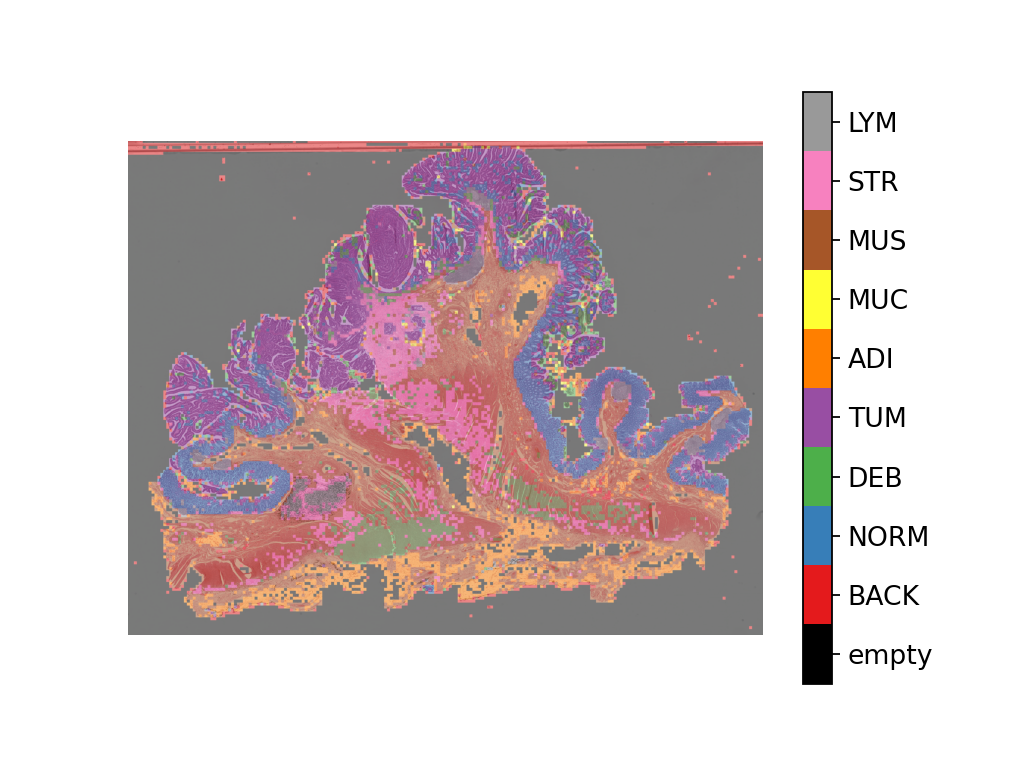
如下所示,將預測地圖疊加在此影像上會得到:
# Visualization of whole-slide image patch-level prediction
# first set up a label to color mapping
label_color_dict = {}
label_color_dict[0] = ("empty", (0, 0, 0))
colors = cm.get_cmap("Set1").colors
for class_name, label in label_dict.items():
    label_color_dict[label + 1] = (class_name, 255 * np.array(colors[label]))

pred_map = predictor.merge_predictions(
    wsi_path,
    wsi_output[0],
    resolution=overview_resolution,
    units=overview_unit,
)
overlay = overlay_prediction_mask(
    wsi_overview,
    pred_map,
    alpha=0.5,
    label_info=label_color_dict,
    return_ax=True,
)
plt.show()
使用病理學特定模型進行特徵提取
在本節中,我們將展示如何使用 TIAToolbox 提供的 WSI 推論引擎,從 TIAToolbox 之外的預訓練 PyTorch 模型中提取特徵。 為了說明這一點,我們將使用 HistoEncoder,這是一個計算病理學特定的模型,經過自我監督的訓練,可以從組織學影像中提取特徵。 該模型已在此處提供:
「HistoEncoder:數位病理學的基礎模型」( https://github.com/jopo666/HistoEncoder ),作者是赫爾辛基大學的 Pohjonen, Joona 及其團隊。
我們將繪製一個特徵圖的 UMAP 降維到 3D (RGB) 中,以可視化這些特徵如何捕捉上述一些組織類型之間的差異。
# Import some extra modules
import histoencoder.functional as F
import torch.nn as nn

from tiatoolbox.models.engine.semantic_segmentor import DeepFeatureExtractor, IOSegmentorConfig
from tiatoolbox.models.models_abc import ModelABC
import umap
TIAToolbox 定義了一個 ModelABC,它是一個繼承 PyTorch nn.Module 的類別,並指定了模型應如何呈現,以便在 TIAToolbox 推論引擎中使用。 histoencoder 模型不遵循此結構,因此我們需要將它包裝在一個類別中,其輸出和方法是 TIAToolbox 引擎所期望的。
class HistoEncWrapper(ModelABC):
    """Wrapper for HistoEnc model that conforms to tiatoolbox ModelABC interface."""

    def __init__(self: HistoEncWrapper, encoder) -> None:
        super().__init__()
        self.feat_extract = encoder

    def forward(self: HistoEncWrapper, imgs: torch.Tensor) -> torch.Tensor:
        """Pass input data through the model.

        Args:
            imgs (torch.Tensor):
                Model input.

        """
        out = F.extract_features(self.feat_extract, imgs, num_blocks=2, avg_pool=True)
        return out

    @staticmethod
    def infer_batch(
        model: nn.Module,
        batch_data: torch.Tensor,
        *,
        on_gpu: bool,
    ) -> list[np.ndarray]:
        """Run inference on an input batch.

        Contains logic for forward operation as well as i/o aggregation.

        Args:
            model (nn.Module):
                PyTorch defined model.
            batch_data (torch.Tensor):
                A batch of data generated by
                `torch.utils.data.DataLoader`.
            on_gpu (bool):
                Whether to run inference on a GPU.

        """
        img_patches_device = batch_data.to('cuda') if on_gpu else batch_data
        model.eval()
        # Do not compute the gradient (not training)
        with torch.inference_mode():
            output = model(img_patches_device)
        return [output.cpu().numpy()]
現在我們有了包裝器,我們將建立我們的特徵提取模型,並實例化一個 DeepFeatureExtractor,以便我們可以在 WSI 上使用這個模型。 我們將使用與上面相同的 WSI,但這次我們將使用 HistoEncoder 模型從 WSI 的圖塊中提取特徵,而不是預測每個圖塊的標籤。
# create the model
encoder = F.create_encoder("prostate_medium")
model = HistoEncWrapper(encoder)

# set the pre-processing function
norm=transforms.Normalize(mean=[0.662, 0.446, 0.605],std=[0.169, 0.190, 0.155])
trans = [
    transforms.ToTensor(),
    norm,
]
model.preproc_func = transforms.Compose(trans)

wsi_ioconfig = IOSegmentorConfig(
    input_resolutions=[{"units": "mpp", "resolution": 0.5}],
    patch_input_shape=[224, 224],
    output_resolutions=[{"units": "mpp", "resolution": 0.5}],
    patch_output_shape=[224, 224],
    stride_shape=[224, 224],
)
當我們建立 DeepFeatureExtractor 時,我們將傳遞 auto_generate_mask=True 參數。 這將使用 otsu 閾值自動建立組織區域的遮罩,以便提取器僅處理包含組織的圖塊。
# create the feature extractor and run it on the WSI
extractor = DeepFeatureExtractor(model=model, auto_generate_mask=True, batch_size=32, num_loader_workers=4, num_postproc_workers=4)
with suppress_console_output():
    out = extractor.predict(imgs=[wsi_path], mode="wsi", ioconfig=wsi_ioconfig, save_dir=global_save_dir / "wsi_features",)
這些特徵可以用來訓練下游模型,但為了了解這些特徵代表什麼,我們將使用 UMAP 降維來可視化 RGB 空間中的特徵。 以相似顏色標記的點應該具有相似的特徵,因此我們可以檢查當我們將 UMAP 降維疊加在 WSI 縮圖上時,這些特徵是否自然地分離成不同的組織區域。 我們將在以下儲存格中將其與上述圖塊層級預測地圖一起繪製,以了解這些特徵如何與圖塊層級預測進行比較。
# First we define a function to calculate the umap reduction
def umap_reducer(x, dims=3, nns=10):
    """UMAP reduction of the input data."""
    reducer = umap.UMAP(n_neighbors=nns, n_components=dims, metric="manhattan", spread=0.5, random_state=2)
    reduced = reducer.fit_transform(x)
    reduced -= reduced.min(axis=0)
    reduced /= reduced.max(axis=0)
    return reduced

# load the features output by our feature extractor
pos = np.load(global_save_dir / "wsi_features" / "0.position.npy")
feats = np.load(global_save_dir / "wsi_features" / "0.features.0.npy")
pos = pos / 8 # as we extracted at 0.5mpp, and we are overlaying on a thumbnail at 4mpp

# reduce the features into 3 dimensional (rgb) space
reduced = umap_reducer(feats)

# plot the prediction map the classifier again
overlay = overlay_prediction_mask(
    wsi_overview,
    pred_map,
    alpha=0.5,
    label_info=label_color_dict,
    return_ax=True,
)

# plot the feature map reduction
plt.figure()
plt.imshow(wsi_overview)
plt.scatter(pos[:,0], pos[:,1], c=reduced, s=1, alpha=0.5)
plt.axis("off")
plt.title("UMAP reduction of HistoEnc features")
plt.show()

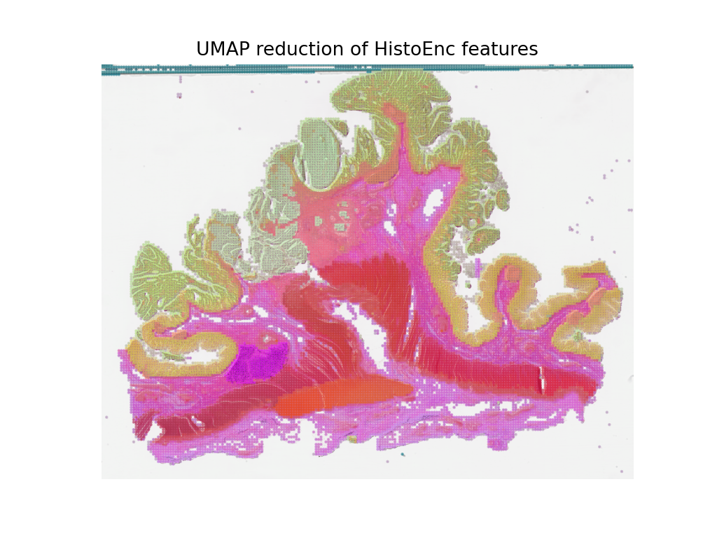
我們看到,來自我們的圖塊層級預測器的預測地圖,以及來自我們的自我監督特徵編碼器的特徵圖,捕捉了關於 WSI 中組織類型的相似資訊。 這是一個很好的完整性檢查,表明我們的模型正在按預期工作。 它還表明,HistoEncoder 模型提取的特徵正在捕捉組織類型之間的差異,因此它們正在編碼組織學相關資訊。
從這裡開始
在本筆記本中,我們展示了如何使用 PatchPredictor 和 DeepFeatureExtractor 類別及其 predict 方法來預測標籤,或提取大圖塊和 WSI 圖塊的特徵。 我們介紹了 merge_predictions 和 overlay_prediction_mask 輔助函數,它們合併圖塊預測輸出,並將結果預測地圖可視化為輸入影像/WSI 上的疊加層。
所有過程都在 TIAToolbox 中進行,我們可以輕鬆地按照我們的範例程式碼將各個部分組裝在一起。 請確保正確設定輸入和選項。 我們鼓勵您進一步研究更改 predict 函數參數對預測輸出的影響。 我們已經示範了如何使用您自己的預訓練模型或研究社群提供的模型來執行 TIAToolbox 框架中特定任務的大型 WSI 推論,即使該模型結構未在 TIAToolbox 模型類別中定義。
您可以透過以下資源了解更多資訊:
