


注意
點擊此處下載完整範例程式碼
空間轉換器網路教學
建立於:2017 年 11 月 08 日 | 最後更新:2024 年 1 月 19 日 | 最後驗證:2024 年 11 月 05 日
作者: Ghassen HAMROUNI
在本教學中,您將學習如何使用稱為空間轉換器網路的視覺注意力機制來擴充您的網路。您可以在 DeepMind 論文中閱讀更多關於空間轉換器網路的資訊
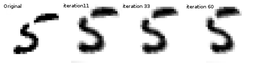
空間轉換器網路是可微分注意力對於任何空間轉換的概括。空間轉換器網路(簡稱 STN)允許神經網路學習如何對輸入影像執行空間轉換,以增強模型的幾何不變性。例如,它可以裁剪感興趣的區域、縮放並校正影像的方向。這可能是一個有用的機制,因為 CNN 對於旋轉和縮放以及更一般的仿射轉換是不變的。
關於 STN 最好的事情之一就是能夠以非常小的修改將其簡單地插入到任何現有的 CNN 中。
# License: BSD
# Author: Ghassen Hamrouni

import torch
import torch.nn as nn
import torch.nn.functional as F
import torch.optim as optim
import torchvision
from torchvision import datasets, transforms
import matplotlib.pyplot as plt
import numpy as np

plt.ion()   # interactive mode
<contextlib.ExitStack object at 0x7f05e9e6ee30>
載入資料
在這篇文章中,我們嘗試使用經典的 MNIST 資料集。使用標準卷積網路並以空間轉換器網路擴充。
from six.moves import urllib
opener = urllib.request.build_opener()
opener.addheaders = [('User-agent', 'Mozilla/5.0')]
urllib.request.install_opener(opener)

device = torch.device("cuda" if torch.cuda.is_available() else "cpu")

# Training dataset
train_loader = torch.utils.data.DataLoader(
    datasets.MNIST(root='.', train=True, download=True,
                   transform=transforms.Compose([
                       transforms.ToTensor(),
                       transforms.Normalize((0.1307,), (0.3081,))
                   ])), batch_size=64, shuffle=True, num_workers=4)
# Test dataset
test_loader = torch.utils.data.DataLoader(
    datasets.MNIST(root='.', train=False, transform=transforms.Compose([
        transforms.ToTensor(),
        transforms.Normalize((0.1307,), (0.3081,))
    ])), batch_size=64, shuffle=True, num_workers=4)
  0%|          | 0.00/9.91M [00:00<?, ?B/s]
100%|##########| 9.91M/9.91M [00:00<00:00, 135MB/s]

  0%|          | 0.00/28.9k [00:00<?, ?B/s]
100%|##########| 28.9k/28.9k [00:00<00:00, 103MB/s]

  0%|          | 0.00/1.65M [00:00<?, ?B/s]
100%|##########| 1.65M/1.65M [00:00<00:00, 329MB/s]

  0%|          | 0.00/4.54k [00:00<?, ?B/s]
100%|##########| 4.54k/4.54k [00:00<00:00, 22.2MB/s]
描述空間轉換器網路
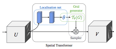
空間轉換器網路歸結為三個主要組成部分
定位網路是一個常規的 CNN,它回歸轉換參數。轉換永遠不會從這個資料集中顯式學習,相反,網路會自動學習空間轉換,從而提高整體準確性。
網格產生器在輸入影像中產生與輸出影像中每個像素相對應的座標網格。
取樣器使用轉換的參數並將其應用於輸入影像。
注意
我們需要包含 affine_grid 和 grid_sample 模組的最新版 PyTorch。
class Net(nn.Module):
    def __init__(self):
        super(Net, self).__init__()
        self.conv1 = nn.Conv2d(1, 10, kernel_size=5)
        self.conv2 = nn.Conv2d(10, 20, kernel_size=5)
        self.conv2_drop = nn.Dropout2d()
        self.fc1 = nn.Linear(320, 50)
        self.fc2 = nn.Linear(50, 10)

        # Spatial transformer localization-network
        self.localization = nn.Sequential(
            nn.Conv2d(1, 8, kernel_size=7),
            nn.MaxPool2d(2, stride=2),
            nn.ReLU(True),
            nn.Conv2d(8, 10, kernel_size=5),
            nn.MaxPool2d(2, stride=2),
            nn.ReLU(True)
        )

        # Regressor for the 3 * 2 affine matrix
        self.fc_loc = nn.Sequential(
            nn.Linear(10 * 3 * 3, 32),
            nn.ReLU(True),
            nn.Linear(32, 3 * 2)
        )

        # Initialize the weights/bias with identity transformation
        self.fc_loc[2].weight.data.zero_()
        self.fc_loc[2].bias.data.copy_(torch.tensor([1, 0, 0, 0, 1, 0], dtype=torch.float))

    # Spatial transformer network forward function
    def stn(self, x):
        xs = self.localization(x)
        xs = xs.view(-1, 10 * 3 * 3)
        theta = self.fc_loc(xs)
        theta = theta.view(-1, 2, 3)

        grid = F.affine_grid(theta, x.size())
        x = F.grid_sample(x, grid)

        return x

    def forward(self, x):
        # transform the input
        x = self.stn(x)

        # Perform the usual forward pass
        x = F.relu(F.max_pool2d(self.conv1(x), 2))
        x = F.relu(F.max_pool2d(self.conv2_drop(self.conv2(x)), 2))
        x = x.view(-1, 320)
        x = F.relu(self.fc1(x))
        x = F.dropout(x, training=self.training)
        x = self.fc2(x)
        return F.log_softmax(x, dim=1)


model = Net().to(device)
訓練模型
現在,讓我們使用 SGD 演算法來訓練模型。該網路正在以監督的方式學習分類任務。同時,該模型正在以端對端的方式自動學習 STN。
optimizer = optim.SGD(model.parameters(), lr=0.01)


def train(epoch):
    model.train()
    for batch_idx, (data, target) in enumerate(train_loader):
        data, target = data.to(device), target.to(device)

        optimizer.zero_grad()
        output = model(data)
        loss = F.nll_loss(output, target)
        loss.backward()
        optimizer.step()
        if batch_idx % 500 == 0:
            print('Train Epoch: {} [{}/{} ({:.0f}%)]\tLoss: {:.6f}'.format(
                epoch, batch_idx * len(data), len(train_loader.dataset),
                100. * batch_idx / len(train_loader), loss.item()))
#
# A simple test procedure to measure the STN performances on MNIST.
#


def test():
    with torch.no_grad():
        model.eval()
        test_loss = 0
        correct = 0
        for data, target in test_loader:
            data, target = data.to(device), target.to(device)
            output = model(data)

            # sum up batch loss
            test_loss += F.nll_loss(output, target, size_average=False).item()
            # get the index of the max log-probability
            pred = output.max(1, keepdim=True)[1]
            correct += pred.eq(target.view_as(pred)).sum().item()

        test_loss /= len(test_loader.dataset)
        print('\nTest set: Average loss: {:.4f}, Accuracy: {}/{} ({:.0f}%)\n'
              .format(test_loss, correct, len(test_loader.dataset),
                      100. * correct / len(test_loader.dataset)))
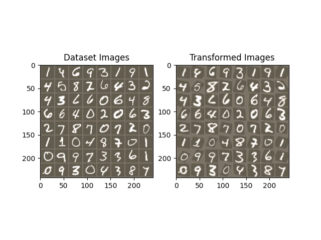
視覺化 STN 結果
現在,我們將檢查我們學習到的視覺注意力機制的結果。
我們定義一個小的輔助函數,以便在訓練時視覺化轉換。
def convert_image_np(inp):
    """Convert a Tensor to numpy image."""
    inp = inp.numpy().transpose((1, 2, 0))
    mean = np.array([0.485, 0.456, 0.406])
    std = np.array([0.229, 0.224, 0.225])
    inp = std * inp + mean
    inp = np.clip(inp, 0, 1)
    return inp

# We want to visualize the output of the spatial transformers layer
# after the training, we visualize a batch of input images and
# the corresponding transformed batch using STN.


def visualize_stn():
    with torch.no_grad():
        # Get a batch of training data
        data = next(iter(test_loader))[0].to(device)

        input_tensor = data.cpu()
        transformed_input_tensor = model.stn(data).cpu()

        in_grid = convert_image_np(
            torchvision.utils.make_grid(input_tensor))

        out_grid = convert_image_np(
            torchvision.utils.make_grid(transformed_input_tensor))

        # Plot the results side-by-side
        f, axarr = plt.subplots(1, 2)
        axarr[0].imshow(in_grid)
        axarr[0].set_title('Dataset Images')

        axarr[1].imshow(out_grid)
        axarr[1].set_title('Transformed Images')

for epoch in range(1, 20 + 1):
    train(epoch)
    test()

# Visualize the STN transformation on some input batch
visualize_stn()

plt.ioff()
plt.show()
/usr/local/lib/python3.10/dist-packages/torch/nn/functional.py:5082: UserWarning:

Default grid_sample and affine_grid behavior has changed to align_corners=False since 1.3.0. Please specify align_corners=True if the old behavior is desired. See the documentation of grid_sample for details.

/usr/local/lib/python3.10/dist-packages/torch/nn/functional.py:5015: UserWarning:

Default grid_sample and affine_grid behavior has changed to align_corners=False since 1.3.0. Please specify align_corners=True if the old behavior is desired. See the documentation of grid_sample for details.

Train Epoch: 1 [0/60000 (0%)]   Loss: 2.315648
Train Epoch: 1 [32000/60000 (53%)]      Loss: 1.070991
/usr/local/lib/python3.10/dist-packages/torch/nn/_reduction.py:51: UserWarning:

size_average and reduce args will be deprecated, please use reduction='sum' instead.


Test set: Average loss: 0.2540, Accuracy: 9309/10000 (93%)

Train Epoch: 2 [0/60000 (0%)]   Loss: 0.547254
Train Epoch: 2 [32000/60000 (53%)]      Loss: 0.306006

Test set: Average loss: 0.1548, Accuracy: 9545/10000 (95%)

Train Epoch: 3 [0/60000 (0%)]   Loss: 0.346975
Train Epoch: 3 [32000/60000 (53%)]      Loss: 0.237371

Test set: Average loss: 0.1362, Accuracy: 9579/10000 (96%)

Train Epoch: 4 [0/60000 (0%)]   Loss: 0.410911
Train Epoch: 4 [32000/60000 (53%)]      Loss: 0.143433

Test set: Average loss: 0.1182, Accuracy: 9656/10000 (97%)

Train Epoch: 5 [0/60000 (0%)]   Loss: 0.232937
Train Epoch: 5 [32000/60000 (53%)]      Loss: 0.201194

Test set: Average loss: 0.2206, Accuracy: 9347/10000 (93%)

Train Epoch: 6 [0/60000 (0%)]   Loss: 0.441828
Train Epoch: 6 [32000/60000 (53%)]      Loss: 0.130507

Test set: Average loss: 0.0715, Accuracy: 9791/10000 (98%)

Train Epoch: 7 [0/60000 (0%)]   Loss: 0.089327
Train Epoch: 7 [32000/60000 (53%)]      Loss: 0.189949

Test set: Average loss: 0.0669, Accuracy: 9801/10000 (98%)

Train Epoch: 8 [0/60000 (0%)]   Loss: 0.213020
Train Epoch: 8 [32000/60000 (53%)]      Loss: 0.126238

Test set: Average loss: 0.0647, Accuracy: 9810/10000 (98%)

Train Epoch: 9 [0/60000 (0%)]   Loss: 0.078002
Train Epoch: 9 [32000/60000 (53%)]      Loss: 0.104715

Test set: Average loss: 0.0741, Accuracy: 9776/10000 (98%)

Train Epoch: 10 [0/60000 (0%)]  Loss: 0.138969
Train Epoch: 10 [32000/60000 (53%)]     Loss: 0.205099

Test set: Average loss: 0.0535, Accuracy: 9828/10000 (98%)

Train Epoch: 11 [0/60000 (0%)]  Loss: 0.170541
Train Epoch: 11 [32000/60000 (53%)]     Loss: 0.079690

Test set: Average loss: 0.0662, Accuracy: 9808/10000 (98%)

Train Epoch: 12 [0/60000 (0%)]  Loss: 0.121953
Train Epoch: 12 [32000/60000 (53%)]     Loss: 0.219585

Test set: Average loss: 0.0606, Accuracy: 9801/10000 (98%)

Train Epoch: 13 [0/60000 (0%)]  Loss: 0.085162
Train Epoch: 13 [32000/60000 (53%)]     Loss: 0.081327

Test set: Average loss: 0.0591, Accuracy: 9819/10000 (98%)

Train Epoch: 14 [0/60000 (0%)]  Loss: 0.060252
Train Epoch: 14 [32000/60000 (53%)]     Loss: 0.164528

Test set: Average loss: 0.0508, Accuracy: 9858/10000 (99%)

Train Epoch: 15 [0/60000 (0%)]  Loss: 0.037811
Train Epoch: 15 [32000/60000 (53%)]     Loss: 0.106973

Test set: Average loss: 0.0456, Accuracy: 9872/10000 (99%)

Train Epoch: 16 [0/60000 (0%)]  Loss: 0.055275
Train Epoch: 16 [32000/60000 (53%)]     Loss: 0.125036

Test set: Average loss: 0.0465, Accuracy: 9864/10000 (99%)

Train Epoch: 17 [0/60000 (0%)]  Loss: 0.265591
Train Epoch: 17 [32000/60000 (53%)]     Loss: 0.253517

Test set: Average loss: 0.0596, Accuracy: 9828/10000 (98%)

Train Epoch: 18 [0/60000 (0%)]  Loss: 0.049595
Train Epoch: 18 [32000/60000 (53%)]     Loss: 0.096609

Test set: Average loss: 0.0516, Accuracy: 9853/10000 (99%)

Train Epoch: 19 [0/60000 (0%)]  Loss: 0.081379
Train Epoch: 19 [32000/60000 (53%)]     Loss: 0.112759

Test set: Average loss: 0.0464, Accuracy: 9856/10000 (99%)

Train Epoch: 20 [0/60000 (0%)]  Loss: 0.084578
Train Epoch: 20 [32000/60000 (53%)]     Loss: 0.020460

Test set: Average loss: 0.0534, Accuracy: 9842/10000 (98%)
腳本的總執行時間: (2 分鐘 26.045 秒)
