注意

點擊這裡下載完整的範例程式碼

使用 TorchRL 的強化學習 (PPO) 教學¶

建立於：2023 年 3 月 15 日 | 最後更新：2025 年 1 月 27 日 | 最後驗證：2024 年 11 月 05 日

作者：Vincent Moens

本教學展示如何使用 PyTorch 和 torchrl 來訓練參數化策略網路，以解決來自 OpenAI-Gym/Farama-Gymnasium 控制函式庫的倒立單擺任務。

倒立單擺¶

主要學習內容

如何在 TorchRL 中建立環境、轉換其輸出，並從該環境收集資料；
如何使用 TensorDict 使您的類別彼此溝通；
使用 TorchRL 建立訓練迴圈的基本知識
- 如何計算策略梯度方法的優勢訊號；
- 如何使用機率神經網路建立隨機策略；
- 如何建立動態重播緩衝區並從中採樣而不重複。

我們將涵蓋 TorchRL 的六個關鍵元件

如果您在 Google Colab 中執行此程式碼，請確保您安裝了以下相依性

!pip3 install torchrl
!pip3 install gym[mujoco]
!pip3 install tqdm

近端策略最佳化 (Proximal Policy Optimization, PPO) 是一種策略梯度演算法，其中收集一批資料並直接用於訓練策略，以最大化給定一些鄰近性約束的預期回報。您可以將其視為 REINFORCE 的複雜版本，REINFORCE 是基礎策略最佳化演算法。如需更多資訊，請參閱近端策略最佳化演算法論文。

PPO 通常被認為是一種快速有效的方法，適用於線上、基於策略的強化學習演算法。 TorchRL 提供了一個損失模組，可以為您完成所有工作，因此您可以依賴此實作，並專注於解決您的問題，而不是每次想要訓練策略時都重新發明輪子。

為了完整起見，以下簡要概述了損失的計算方式，即使這由我們的 ClipPPOLoss 模組負責—該演算法的工作方式如下：1. 我們將透過在環境中執行策略給定的步數來採樣一批資料。 2. 然後，我們將使用 REINFORCE 損失的剪裁版本，對此批次進行給定數量的具有隨機子樣本的最佳化步驟。 3. 剪裁將對我們的損失設定一個悲觀的界限：與較高的估計相比，較低的返回估計將受到青睞。損失的精確公式是

\[L(s,a,\theta_k,\theta) = \min\left( \frac{\pi_{\theta}(a|s)}{\pi_{\theta_k}(a|s)} A^{\pi_{\theta_k}}(s,a), \;\; g(\epsilon, A^{\pi_{\theta_k}}(s,a)) \right),\]

該損失有兩個組成部分：在最小運算符的第一部分中，我們只是計算 REINFORCE 損失的加權重要性版本（例如，我們針對目前策略配置滯後於用於資料收集的配置的事實進行校正的 REINFORCE 損失）。最小運算符的第二部分是類似的損失，其中當比率超過或低於給定的一對閾值時，我們剪裁了這些比率。

此損失確保無論優勢是正數還是負數，都會阻止產生與先前配置顯著轉變的策略更新。

本教學的結構如下

首先，我們將定義一組用於訓練的超參數。
接下來，我們將專注於使用 TorchRL 的包裝器和轉換來建立我們的環境或模擬器。
接下來，我們將設計策略網路和價值模型，這對於損失函數是不可或缺的。這些模組將用於配置我們的損失模組。
接下來，我們將建立重播緩衝區和資料載入器。
最後，我們將執行我們的訓練迴圈並分析結果。

在本教學中，我們將使用 tensordict 函式庫。 TensorDict 是 TorchRL 的通用語言：它有助於我們抽象模組的讀取和寫入內容，並且更關心演算法本身，而較少關心特定的資料描述。

import warnings
warnings.filterwarnings("ignore")
from torch import multiprocessing


from collections import defaultdict

import matplotlib.pyplot as plt
import torch
from tensordict.nn import TensorDictModule
from tensordict.nn.distributions import NormalParamExtractor
from torch import nn
from torchrl.collectors import SyncDataCollector
from torchrl.data.replay_buffers import ReplayBuffer
from torchrl.data.replay_buffers.samplers import SamplerWithoutReplacement
from torchrl.data.replay_buffers.storages import LazyTensorStorage
from torchrl.envs import (Compose, DoubleToFloat, ObservationNorm, StepCounter,
                          TransformedEnv)
from torchrl.envs.libs.gym import GymEnv
from torchrl.envs.utils import check_env_specs, ExplorationType, set_exploration_type
from torchrl.modules import ProbabilisticActor, TanhNormal, ValueOperator
from torchrl.objectives import ClipPPOLoss
from torchrl.objectives.value import GAE
from tqdm import tqdm

定義超參數¶

我們設定演算法的超參數。根據可用的資源，可以選擇在 GPU 或另一個裝置上執行策略。 frame_skip 將控制單個動作被執行的幀數。其餘的幀數參數必須針對此值進行校正（因為一個環境步驟實際上將返回 frame_skip 幀）。

is_fork = multiprocessing.get_start_method() == "fork"
device = (
    torch.device(0)
    if torch.cuda.is_available() and not is_fork
    else torch.device("cpu")
)
num_cells = 256  # number of cells in each layer i.e. output dim.
lr = 3e-4
max_grad_norm = 1.0

資料收集參數¶

收集資料時，我們可以透過定義 frames_per_batch 參數來選擇每個批次的大小。我們還將定義允許自己使用的幀數（例如與模擬器的互動次數）。通常，RL 演算法的目標是以環境互動的速度盡快學習解決任務：total_frames 越低越好。

frames_per_batch = 1000
# For a complete training, bring the number of frames up to 1M
total_frames = 50_000

PPO 參數¶

在每次資料收集（或批次收集）時，我們將針對特定數量的epochs執行優化，每次都在巢狀訓練迴圈中消耗我們剛獲得的完整資料。此處的 sub_batch_size 與上面的 frames_per_batch 不同：回想一下，我們正在處理來自我們收集器的「一批資料」，其大小由 frames_per_batch 定義，我們將在內部訓練迴圈中進一步將其分割成更小的子批次。這些子批次的大小由 sub_batch_size 控制。

sub_batch_size = 64  # cardinality of the sub-samples gathered from the current data in the inner loop
num_epochs = 10  # optimization steps per batch of data collected
clip_epsilon = (
    0.2  # clip value for PPO loss: see the equation in the intro for more context.
)
gamma = 0.99
lmbda = 0.95
entropy_eps = 1e-4

定義一個環境¶

在 RL 中，環境通常是我們指代模擬器或控制系統的方式。各種函式庫為強化學習提供模擬環境，包括 Gymnasium（先前為 OpenAI Gym）、DeepMind 控制套件等等。作為一個通用函式庫，TorchRL 的目標是為大量的 RL 模擬器提供一個可互換的介面，讓您可以輕鬆地交換一個環境與另一個環境。例如，可以使用幾個字元建立一個包裝的 gym 環境

base_env = GymEnv("InvertedDoublePendulum-v4", device=device)

在這段程式碼中，有幾件事需要注意：首先，我們透過呼叫 GymEnv 包裝器來建立環境。如果傳遞額外的關鍵字參數，它們將被傳遞到 gym.make 方法，因此涵蓋了最常見的環境建構命令。或者，也可以直接使用 gym.make(env_name, **kwargs) 建立一個 gym 環境，並將其包裝在 GymWrapper 類別中。

還有 device 參數：對於 gym，這只控制輸入動作和觀察到的狀態將被儲存的裝置，但執行將始終在 CPU 上完成。這樣做的原因是 gym 不支援裝置上的執行，除非另有規定。對於其他函式庫，我們可以控制執行裝置，並且盡可能地嘗試在儲存和執行後端保持一致。

轉換¶

我們將在我們的環境中附加一些轉換，以準備策略的資料。在 Gym 中，這通常透過包裝器來實現。TorchRL 採用不同的方法，更類似於其他 pytorch 網域函式庫，透過使用轉換。若要將轉換新增到環境，應該簡單地將其包裝在 TransformedEnv 實例中，並將轉換序列附加到其中。轉換後的環境將繼承包裝環境的裝置和元數據，並根據其包含的轉換序列轉換這些數據。

正規化¶

第一個要編碼的是正規化轉換。作為經驗法則，最好讓資料大致符合單位高斯分佈：為了獲得此結果，我們將在環境中執行一定數量的隨機步驟，並計算這些觀察的摘要統計資料。

我們將附加另外兩個轉換：DoubleToFloat 轉換會將雙精度條目轉換為單精度數字，以便策略讀取。StepCounter 轉換將用於計算環境終止前的步驟數。我們將使用此度量作為效能的補充度量。

正如我們稍後將看到的，許多 TorchRL 的類別都依賴 TensorDict 進行通訊。您可以將其視為具有一些額外張量功能的 python 字典。實際上，這意味著我們將使用的許多模組需要被告知要在它們將接收的 tensordict 中讀取哪個鍵 (in_keys) 以及寫入哪個鍵 (out_keys)。通常，如果省略 out_keys，則假定 in_keys 條目將就地更新。對於我們的轉換，我們唯一感興趣的條目稱為 "observation"，我們的轉換層將被告知僅修改此條目。

env = TransformedEnv(
    base_env,
    Compose(
        # normalize observations
        ObservationNorm(in_keys=["observation"]),
        DoubleToFloat(),
        StepCounter(),
    ),
)

您可能已經注意到，我們建立了一個正規化層，但我們沒有設定其正規化參數。為此，ObservationNorm 可以自動收集我們環境的摘要統計資料

env.transform[0].init_stats(num_iter=1000, reduce_dim=0, cat_dim=0)

ObservationNorm 轉換現在已填充位置和縮放比例，這些將用於正規化資料。

讓我們對摘要統計資料的形狀進行一些健全性檢查

print("normalization constant shape:", env.transform[0].loc.shape)

normalization constant shape: torch.Size([11])

環境不僅由其模擬器和轉換定義，還由一系列元數據定義，這些元數據描述了在其執行期間可以預期的事情。為了提高效率，TorchRL 在環境規格方面非常嚴格，但您可以輕鬆檢查您的環境規格是否足夠。在我們的範例中，繼承自它的 GymWrapper 和 GymEnv 已經負責為您的環境設定正確的規格，因此您不必擔心這一點。

儘管如此，讓我們透過查看其規格來看看使用轉換後的環境的具體範例。有三個規格需要查看：observation_spec，它定義了在環境中執行動作時預期會發生的情況，reward_spec，它指示獎勵網域，最後是 input_spec（其中包含 action_spec），它代表環境執行單一步驟所需的一切。

print("observation_spec:", env.observation_spec)
print("reward_spec:", env.reward_spec)
print("input_spec:", env.input_spec)
print("action_spec (as defined by input_spec):", env.action_spec)

observation_spec: Composite(
    observation: UnboundedContinuous(
        shape=torch.Size([11]),
        space=ContinuousBox(
            low=Tensor(shape=torch.Size([11]), device=cpu, dtype=torch.float32, contiguous=True),
            high=Tensor(shape=torch.Size([11]), device=cpu, dtype=torch.float32, contiguous=True)),
        device=cpu,
        dtype=torch.float32,
        domain=continuous),
    step_count: BoundedDiscrete(
        shape=torch.Size([1]),
        space=ContinuousBox(
            low=Tensor(shape=torch.Size([1]), device=cpu, dtype=torch.int64, contiguous=True),
            high=Tensor(shape=torch.Size([1]), device=cpu, dtype=torch.int64, contiguous=True)),
        device=cpu,
        dtype=torch.int64,
        domain=discrete),
    device=cpu,
    shape=torch.Size([]))
reward_spec: UnboundedContinuous(
    shape=torch.Size([1]),
    space=ContinuousBox(
        low=Tensor(shape=torch.Size([1]), device=cpu, dtype=torch.float32, contiguous=True),
        high=Tensor(shape=torch.Size([1]), device=cpu, dtype=torch.float32, contiguous=True)),
    device=cpu,
    dtype=torch.float32,
    domain=continuous)
input_spec: Composite(
    full_state_spec: Composite(
        step_count: BoundedDiscrete(
            shape=torch.Size([1]),
            space=ContinuousBox(
                low=Tensor(shape=torch.Size([1]), device=cpu, dtype=torch.int64, contiguous=True),
                high=Tensor(shape=torch.Size([1]), device=cpu, dtype=torch.int64, contiguous=True)),
            device=cpu,
            dtype=torch.int64,
            domain=discrete),
        device=cpu,
        shape=torch.Size([])),
    full_action_spec: Composite(
        action: BoundedContinuous(
            shape=torch.Size([1]),
            space=ContinuousBox(
                low=Tensor(shape=torch.Size([1]), device=cpu, dtype=torch.float32, contiguous=True),
                high=Tensor(shape=torch.Size([1]), device=cpu, dtype=torch.float32, contiguous=True)),
            device=cpu,
            dtype=torch.float32,
            domain=continuous),
        device=cpu,
        shape=torch.Size([])),
    device=cpu,
    shape=torch.Size([]))
action_spec (as defined by input_spec): BoundedContinuous(
    shape=torch.Size([1]),
    space=ContinuousBox(
        low=Tensor(shape=torch.Size([1]), device=cpu, dtype=torch.float32, contiguous=True),
        high=Tensor(shape=torch.Size([1]), device=cpu, dtype=torch.float32, contiguous=True)),
    device=cpu,
    dtype=torch.float32,
    domain=continuous)

check_env_specs() 函式執行一個小的 rollout 並將其輸出與環境規格進行比較。如果沒有引發錯誤，我們可以確信規格已正確定義

check_env_specs(env)

為了好玩，讓我們看看一個簡單的隨機 rollout 是什麼樣子。您可以呼叫 env.rollout(n_steps) 並概述環境輸入和輸出的外觀。動作將自動從動作規格網域中繪製，因此您無需擔心設計隨機取樣器。

通常，在每個步驟中，RL 環境會接收一個 action 作為輸入，並輸出一個 observation、一個 reward 和一個 done 狀態。observation 可能是複合式的，意味著它可以由多個張量組成。這對 TorchRL 來說不是問題，因為整組 observations 會自動打包到輸出的 TensorDict 中。在給定步數上執行 rollout (例如，一系列環境步驟和隨機 action 生成) 後，我們將檢索一個 TensorDict 實例，其形狀與此軌跡長度匹配。

rollout = env.rollout(3)
print("rollout of three steps:", rollout)
print("Shape of the rollout TensorDict:", rollout.batch_size)

rollout of three steps: TensorDict(
    fields={
        action: Tensor(shape=torch.Size([3, 1]), device=cpu, dtype=torch.float32, is_shared=False),
        done: Tensor(shape=torch.Size([3, 1]), device=cpu, dtype=torch.bool, is_shared=False),
        next: TensorDict(
            fields={
                done: Tensor(shape=torch.Size([3, 1]), device=cpu, dtype=torch.bool, is_shared=False),
                observation: Tensor(shape=torch.Size([3, 11]), device=cpu, dtype=torch.float32, is_shared=False),
                reward: Tensor(shape=torch.Size([3, 1]), device=cpu, dtype=torch.float32, is_shared=False),
                step_count: Tensor(shape=torch.Size([3, 1]), device=cpu, dtype=torch.int64, is_shared=False),
                terminated: Tensor(shape=torch.Size([3, 1]), device=cpu, dtype=torch.bool, is_shared=False),
                truncated: Tensor(shape=torch.Size([3, 1]), device=cpu, dtype=torch.bool, is_shared=False)},
            batch_size=torch.Size([3]),
            device=cpu,
            is_shared=False),
        observation: Tensor(shape=torch.Size([3, 11]), device=cpu, dtype=torch.float32, is_shared=False),
        step_count: Tensor(shape=torch.Size([3, 1]), device=cpu, dtype=torch.int64, is_shared=False),
        terminated: Tensor(shape=torch.Size([3, 1]), device=cpu, dtype=torch.bool, is_shared=False),
        truncated: Tensor(shape=torch.Size([3, 1]), device=cpu, dtype=torch.bool, is_shared=False)},
    batch_size=torch.Size([3]),
    device=cpu,
    is_shared=False)
Shape of the rollout TensorDict: torch.Size([3])

我們的 rollout 資料的形狀為 torch.Size([3])，這與我們運行的步數相符。 "next" 條目指向當前步驟之後的資料。在大多數情況下，時間 t 的 "next" 資料與 t+1 的資料相符，但如果我們使用某些特定轉換 (例如，多步)，則可能不是這種情況。

策略 (Policy)¶

PPO 利用隨機策略來處理探索。這意味著我們的神經網路必須輸出分布的參數，而不是對應於所採取 action 的單個值。

由於資料是連續的，我們使用 Tanh-Normal 分布來遵守 action 空間邊界。TorchRL 提供了這種分布，我們唯一需要關心的是構建一個神經網路，該網路輸出正確數量的參數，以供策略使用 (一個位置或均值，以及一個尺度)。

\[f_{\theta}(\text{observation}) = \mu_{\theta}(\text{observation}), \sigma^{+}_{\theta}(\text{observation})\]

這裡唯一的額外困難是將我們的輸出分成兩個相等的部分，並將第二部分映射到一個嚴格正的空間。

我們分三個步驟設計策略

定義一個神經網路 D_obs -> 2 * D_action。實際上，我們的 loc (mu) 和 scale (sigma) 都具有維度 D_action。
附加一個 NormalParamExtractor 以提取位置和尺度 (例如，將輸入分成兩個相等的部分，並將正變換應用於尺度參數)。
建立一個機率性的 TensorDictModule，它可以產生此分布並從中抽樣。

actor_net = nn.Sequential(
    nn.LazyLinear(num_cells, device=device),
    nn.Tanh(),
    nn.LazyLinear(num_cells, device=device),
    nn.Tanh(),
    nn.LazyLinear(num_cells, device=device),
    nn.Tanh(),
    nn.LazyLinear(2 * env.action_spec.shape[-1], device=device),
    NormalParamExtractor(),
)

為了使策略能夠透過 tensordict 資料載體與環境“對話”，我們將 nn.Module 包裝在 TensorDictModule 中。這個類別會簡單地讀取它所提供的 in_keys，並將輸出就地寫入到已註冊的 out_keys 中。

policy_module = TensorDictModule(
    actor_net, in_keys=["observation"], out_keys=["loc", "scale"]
)

我們現在需要根據我們正態分佈的位置和尺度來建立一個分布。為此，我們指示 ProbabilisticActor 類別建立一個基於位置和尺度參數的 TanhNormal。我們還提供了此分布的最小值和最大值，這些值是從環境規格中收集的。

in_keys 的名稱 (因此也是上面 TensorDictModule 中的 out_keys 的名稱) 不能設定為任意值，因為 TanhNormal 分布建構子會預期 loc 和 scale 關鍵字參數。也就是說，ProbabilisticActor 也接受 Dict[str, str] 類型的 in_keys，其中鍵值對表示每個要使用的關鍵字參數應使用哪個 in_key 字串。

policy_module = ProbabilisticActor(
    module=policy_module,
    spec=env.action_spec,
    in_keys=["loc", "scale"],
    distribution_class=TanhNormal,
    distribution_kwargs={
        "low": env.action_spec.space.low,
        "high": env.action_spec.space.high,
    },
    return_log_prob=True,
    # we'll need the log-prob for the numerator of the importance weights
)

價值網路 (Value network)¶

價值網路是 PPO 算法的一個關鍵組件，即使它在推理時不會被使用。該模組將讀取 observations 並返回對以下軌跡的折扣回報的估計。這使我們可以透過依賴於在訓練期間即時學習的一些效用估計來攤銷學習。我們的價值網路與策略具有相同的結構，但為了簡化起見，我們為其分配自己的一組參數。

value_net = nn.Sequential(
    nn.LazyLinear(num_cells, device=device),
    nn.Tanh(),
    nn.LazyLinear(num_cells, device=device),
    nn.Tanh(),
    nn.LazyLinear(num_cells, device=device),
    nn.Tanh(),
    nn.LazyLinear(1, device=device),
)

value_module = ValueOperator(
    module=value_net,
    in_keys=["observation"],
)

讓我們試試我們的策略和價值模組。正如我們之前所說的，使用 TensorDictModule 可以直接讀取環境的輸出以運行這些模組，因為它們知道要讀取什麼資訊以及將其寫入何處。

print("Running policy:", policy_module(env.reset()))
print("Running value:", value_module(env.reset()))

Running policy: TensorDict(
    fields={
        action: Tensor(shape=torch.Size([1]), device=cpu, dtype=torch.float32, is_shared=False),
        done: Tensor(shape=torch.Size([1]), device=cpu, dtype=torch.bool, is_shared=False),
        loc: Tensor(shape=torch.Size([1]), device=cpu, dtype=torch.float32, is_shared=False),
        observation: Tensor(shape=torch.Size([11]), device=cpu, dtype=torch.float32, is_shared=False),
        sample_log_prob: Tensor(shape=torch.Size([]), device=cpu, dtype=torch.float32, is_shared=False),
        scale: Tensor(shape=torch.Size([1]), device=cpu, dtype=torch.float32, is_shared=False),
        step_count: Tensor(shape=torch.Size([1]), device=cpu, dtype=torch.int64, is_shared=False),
        terminated: Tensor(shape=torch.Size([1]), device=cpu, dtype=torch.bool, is_shared=False),
        truncated: Tensor(shape=torch.Size([1]), device=cpu, dtype=torch.bool, is_shared=False)},
    batch_size=torch.Size([]),
    device=cpu,
    is_shared=False)
Running value: TensorDict(
    fields={
        done: Tensor(shape=torch.Size([1]), device=cpu, dtype=torch.bool, is_shared=False),
        observation: Tensor(shape=torch.Size([11]), device=cpu, dtype=torch.float32, is_shared=False),
        state_value: Tensor(shape=torch.Size([1]), device=cpu, dtype=torch.float32, is_shared=False),
        step_count: Tensor(shape=torch.Size([1]), device=cpu, dtype=torch.int64, is_shared=False),
        terminated: Tensor(shape=torch.Size([1]), device=cpu, dtype=torch.bool, is_shared=False),
        truncated: Tensor(shape=torch.Size([1]), device=cpu, dtype=torch.bool, is_shared=False)},
    batch_size=torch.Size([]),
    device=cpu,
    is_shared=False)

資料收集器 (Data collector)¶

TorchRL 提供了一組 DataCollector 類別。簡而言之，這些類別執行三個操作：重置環境、根據最新的 observation 計算 action、在環境中執行一個步驟，並重複最後兩個步驟，直到環境發出停止訊號 (或達到完成狀態)。

它們允許您控制在每次迭代中收集多少 frame (透過 frames_per_batch 參數)、何時重置環境 (透過 max_frames_per_traj 參數)、在哪個 device 上執行策略等等。它們還被設計為與批次處理和多進程環境有效協作。

最簡單的資料收集器是 SyncDataCollector：它是一個迭代器，您可以使用它來取得給定長度的資料批次，並且一旦收集到總 frame 數 (total_frames) 就會停止。其他資料收集器 (MultiSyncDataCollector 和 MultiaSyncDataCollector) 將在一組多進程 worker 上以同步和非同步方式執行相同的操作。

與之前的策略和環境一樣，資料收集器將傳回 TensorDict 實例，其元素總數與 frames_per_batch 相符。使用 TensorDict 將資料傳遞到訓練迴圈，使您可以編寫 100% 不知道 rollout 內容實際特性的資料載入管道。

collector = SyncDataCollector(
    env,
    policy_module,
    frames_per_batch=frames_per_batch,
    total_frames=total_frames,
    split_trajs=False,
    device=device,
)

回放緩衝區¶

回放緩衝區是離線強化學習演算法中常見的建構元件。在線上策略情境中，回放緩衝區會在每次收集一批資料時重新填充，並且其資料會被重複使用一定次數的 epoch。

TorchRL 的回放緩衝區是使用一個通用的容器 ReplayBuffer 建構的，該容器將緩衝區的元件作為參數：一個儲存器、一個寫入器、一個取樣器，以及可能的一些轉換器。只有儲存器（指示回放緩衝區的容量）是強制性的。我們還指定了一個沒有重複的取樣器，以避免在一個 epoch 中多次取樣相同的項目。對於 PPO 而言，使用回放緩衝區並非強制性的，我們可以簡單地從收集的批次中取樣子批次，但是使用這些類別使我們可以輕鬆地以可重現的方式建構內部訓練迴圈。

replay_buffer = ReplayBuffer(
    storage=LazyTensorStorage(max_size=frames_per_batch),
    sampler=SamplerWithoutReplacement(),
)

損失函數¶

為了方便起見，PPO 損失可以直接從 TorchRL 導入，使用 ClipPPOLoss 類別。這是利用 PPO 最簡單的方法：它隱藏了 PPO 的數學運算和控制流程。

PPO 需要計算一些「優勢估計」。簡而言之，優勢是一個反映回報值期望的數值，同時處理偏差/變異數的權衡。要計算優勢，只需 (1) 建構優勢模組，該模組利用我們的價值運算子，以及 (2) 在每個 epoch 之前，將每個批次的資料傳遞給它。GAE 模組將使用新的 "advantage" 和 "value_target" 條目更新輸入的 tensordict。"value_target" 是一個無梯度張量，代表價值網路應使用輸入觀察表示的經驗價值。這兩者都將被 ClipPPOLoss 用於回傳策略和價值損失。

advantage_module = GAE(
    gamma=gamma, lmbda=lmbda, value_network=value_module, average_gae=True
)

loss_module = ClipPPOLoss(
    actor_network=policy_module,
    critic_network=value_module,
    clip_epsilon=clip_epsilon,
    entropy_bonus=bool(entropy_eps),
    entropy_coef=entropy_eps,
    # these keys match by default but we set this for completeness
    critic_coef=1.0,
    loss_critic_type="smooth_l1",
)

optim = torch.optim.Adam(loss_module.parameters(), lr)
scheduler = torch.optim.lr_scheduler.CosineAnnealingLR(
    optim, total_frames // frames_per_batch, 0.0
)

訓練迴圈¶

我們現在擁有編寫訓練迴圈所需的所有組件。這些步驟包括：

收集資料
- 計算優勢
  - 迴圈遍歷收集的資料以計算損失值
  - 反向傳播
  - 優化
  - 重複
- 重複
重複

logs = defaultdict(list)
pbar = tqdm(total=total_frames)
eval_str = ""

# We iterate over the collector until it reaches the total number of frames it was
# designed to collect:
for i, tensordict_data in enumerate(collector):
    # we now have a batch of data to work with. Let's learn something from it.
    for _ in range(num_epochs):
        # We'll need an "advantage" signal to make PPO work.
        # We re-compute it at each epoch as its value depends on the value
        # network which is updated in the inner loop.
        advantage_module(tensordict_data)
        data_view = tensordict_data.reshape(-1)
        replay_buffer.extend(data_view.cpu())
        for _ in range(frames_per_batch // sub_batch_size):
            subdata = replay_buffer.sample(sub_batch_size)
            loss_vals = loss_module(subdata.to(device))
            loss_value = (
                loss_vals["loss_objective"]
                + loss_vals["loss_critic"]
                + loss_vals["loss_entropy"]
            )

            # Optimization: backward, grad clipping and optimization step
            loss_value.backward()
            # this is not strictly mandatory but it's good practice to keep
            # your gradient norm bounded
            torch.nn.utils.clip_grad_norm_(loss_module.parameters(), max_grad_norm)
            optim.step()
            optim.zero_grad()

    logs["reward"].append(tensordict_data["next", "reward"].mean().item())
    pbar.update(tensordict_data.numel())
    cum_reward_str = (
        f"average reward={logs['reward'][-1]: 4.4f} (init={logs['reward'][0]: 4.4f})"
    )
    logs["step_count"].append(tensordict_data["step_count"].max().item())
    stepcount_str = f"step count (max): {logs['step_count'][-1]}"
    logs["lr"].append(optim.param_groups[0]["lr"])
    lr_str = f"lr policy: {logs['lr'][-1]: 4.4f}"
    if i % 10 == 0:
        # We evaluate the policy once every 10 batches of data.
        # Evaluation is rather simple: execute the policy without exploration
        # (take the expected value of the action distribution) for a given
        # number of steps (1000, which is our ``env`` horizon).
        # The ``rollout`` method of the ``env`` can take a policy as argument:
        # it will then execute this policy at each step.
        with set_exploration_type(ExplorationType.DETERMINISTIC), torch.no_grad():
            # execute a rollout with the trained policy
            eval_rollout = env.rollout(1000, policy_module)
            logs["eval reward"].append(eval_rollout["next", "reward"].mean().item())
            logs["eval reward (sum)"].append(
                eval_rollout["next", "reward"].sum().item()
            )
            logs["eval step_count"].append(eval_rollout["step_count"].max().item())
            eval_str = (
                f"eval cumulative reward: {logs['eval reward (sum)'][-1]: 4.4f} "
                f"(init: {logs['eval reward (sum)'][0]: 4.4f}), "
                f"eval step-count: {logs['eval step_count'][-1]}"
            )
            del eval_rollout
    pbar.set_description(", ".join([eval_str, cum_reward_str, stepcount_str, lr_str]))

    # We're also using a learning rate scheduler. Like the gradient clipping,
    # this is a nice-to-have but nothing necessary for PPO to work.
    scheduler.step()

  0%|          | 0/50000 [00:00<?, ?it/s]
  2%|2         | 1000/50000 [00:04<03:17, 248.03it/s]
eval cumulative reward:  91.9271 (init:  91.9271), eval step-count: 9, average reward= 9.0969 (init= 9.0969), step count (max): 11, lr policy:  0.0003:   2%|2         | 1000/50000 [00:04<03:17, 248.03it/s]
eval cumulative reward:  91.9271 (init:  91.9271), eval step-count: 9, average reward= 9.0969 (init= 9.0969), step count (max): 11, lr policy:  0.0003:   4%|4         | 2000/50000 [00:07<03:09, 253.73it/s]
eval cumulative reward:  91.9271 (init:  91.9271), eval step-count: 9, average reward= 9.1171 (init= 9.0969), step count (max): 16, lr policy:  0.0003:   4%|4         | 2000/50000 [00:07<03:09, 253.73it/s]
eval cumulative reward:  91.9271 (init:  91.9271), eval step-count: 9, average reward= 9.1171 (init= 9.0969), step count (max): 16, lr policy:  0.0003:   6%|6         | 3000/50000 [00:11<03:04, 255.42it/s]
eval cumulative reward:  91.9271 (init:  91.9271), eval step-count: 9, average reward= 9.1550 (init= 9.0969), step count (max): 20, lr policy:  0.0003:   6%|6         | 3000/50000 [00:11<03:04, 255.42it/s]
eval cumulative reward:  91.9271 (init:  91.9271), eval step-count: 9, average reward= 9.1550 (init= 9.0969), step count (max): 20, lr policy:  0.0003:   8%|8         | 4000/50000 [00:15<02:58, 258.33it/s]
eval cumulative reward:  91.9271 (init:  91.9271), eval step-count: 9, average reward= 9.1764 (init= 9.0969), step count (max): 19, lr policy:  0.0003:   8%|8         | 4000/50000 [00:15<02:58, 258.33it/s]
eval cumulative reward:  91.9271 (init:  91.9271), eval step-count: 9, average reward= 9.1764 (init= 9.0969), step count (max): 19, lr policy:  0.0003:  10%|#         | 5000/50000 [00:19<02:52, 260.64it/s]
eval cumulative reward:  91.9271 (init:  91.9271), eval step-count: 9, average reward= 9.2009 (init= 9.0969), step count (max): 26, lr policy:  0.0003:  10%|#         | 5000/50000 [00:19<02:52, 260.64it/s]
eval cumulative reward:  91.9271 (init:  91.9271), eval step-count: 9, average reward= 9.2009 (init= 9.0969), step count (max): 26, lr policy:  0.0003:  12%|#2        | 6000/50000 [00:23<02:47, 262.48it/s]
eval cumulative reward:  91.9271 (init:  91.9271), eval step-count: 9, average reward= 9.2242 (init= 9.0969), step count (max): 26, lr policy:  0.0003:  12%|#2        | 6000/50000 [00:23<02:47, 262.48it/s]
eval cumulative reward:  91.9271 (init:  91.9271), eval step-count: 9, average reward= 9.2242 (init= 9.0969), step count (max): 26, lr policy:  0.0003:  14%|#4        | 7000/50000 [00:26<02:43, 263.76it/s]
eval cumulative reward:  91.9271 (init:  91.9271), eval step-count: 9, average reward= 9.2368 (init= 9.0969), step count (max): 30, lr policy:  0.0003:  14%|#4        | 7000/50000 [00:26<02:43, 263.76it/s]
eval cumulative reward:  91.9271 (init:  91.9271), eval step-count: 9, average reward= 9.2368 (init= 9.0969), step count (max): 30, lr policy:  0.0003:  16%|#6        | 8000/50000 [00:30<02:38, 265.00it/s]
eval cumulative reward:  91.9271 (init:  91.9271), eval step-count: 9, average reward= 9.2486 (init= 9.0969), step count (max): 46, lr policy:  0.0003:  16%|#6        | 8000/50000 [00:30<02:38, 265.00it/s]
eval cumulative reward:  91.9271 (init:  91.9271), eval step-count: 9, average reward= 9.2486 (init= 9.0969), step count (max): 46, lr policy:  0.0003:  18%|#8        | 9000/50000 [00:34<02:37, 259.69it/s]
eval cumulative reward:  91.9271 (init:  91.9271), eval step-count: 9, average reward= 9.2509 (init= 9.0969), step count (max): 47, lr policy:  0.0003:  18%|#8        | 9000/50000 [00:34<02:37, 259.69it/s]
eval cumulative reward:  91.9271 (init:  91.9271), eval step-count: 9, average reward= 9.2509 (init= 9.0969), step count (max): 47, lr policy:  0.0003:  20%|##        | 10000/50000 [00:38<02:32, 262.13it/s]
eval cumulative reward:  91.9271 (init:  91.9271), eval step-count: 9, average reward= 9.2599 (init= 9.0969), step count (max): 52, lr policy:  0.0003:  20%|##        | 10000/50000 [00:38<02:32, 262.13it/s]
eval cumulative reward:  91.9271 (init:  91.9271), eval step-count: 9, average reward= 9.2599 (init= 9.0969), step count (max): 52, lr policy:  0.0003:  22%|##2       | 11000/50000 [00:42<02:27, 263.79it/s]
eval cumulative reward:  371.6797 (init:  91.9271), eval step-count: 39, average reward= 9.2698 (init= 9.0969), step count (max): 56, lr policy:  0.0003:  22%|##2       | 11000/50000 [00:42<02:27, 263.79it/s]
eval cumulative reward:  371.6797 (init:  91.9271), eval step-count: 39, average reward= 9.2698 (init= 9.0969), step count (max): 56, lr policy:  0.0003:  24%|##4       | 12000/50000 [00:45<02:24, 263.22it/s]
eval cumulative reward:  371.6797 (init:  91.9271), eval step-count: 39, average reward= 9.2751 (init= 9.0969), step count (max): 75, lr policy:  0.0003:  24%|##4       | 12000/50000 [00:45<02:24, 263.22it/s]
eval cumulative reward:  371.6797 (init:  91.9271), eval step-count: 39, average reward= 9.2751 (init= 9.0969), step count (max): 75, lr policy:  0.0003:  26%|##6       | 13000/50000 [00:49<02:19, 264.82it/s]
eval cumulative reward:  371.6797 (init:  91.9271), eval step-count: 39, average reward= 9.2811 (init= 9.0969), step count (max): 92, lr policy:  0.0003:  26%|##6       | 13000/50000 [00:49<02:19, 264.82it/s]
eval cumulative reward:  371.6797 (init:  91.9271), eval step-count: 39, average reward= 9.2811 (init= 9.0969), step count (max): 92, lr policy:  0.0003:  28%|##8       | 14000/50000 [00:53<02:15, 265.99it/s]
eval cumulative reward:  371.6797 (init:  91.9271), eval step-count: 39, average reward= 9.2798 (init= 9.0969), step count (max): 75, lr policy:  0.0003:  28%|##8       | 14000/50000 [00:53<02:15, 265.99it/s]
eval cumulative reward:  371.6797 (init:  91.9271), eval step-count: 39, average reward= 9.2798 (init= 9.0969), step count (max): 75, lr policy:  0.0003:  30%|###       | 15000/50000 [00:57<02:11, 266.73it/s]
eval cumulative reward:  371.6797 (init:  91.9271), eval step-count: 39, average reward= 9.2881 (init= 9.0969), step count (max): 64, lr policy:  0.0002:  30%|###       | 15000/50000 [00:57<02:11, 266.73it/s]
eval cumulative reward:  371.6797 (init:  91.9271), eval step-count: 39, average reward= 9.2881 (init= 9.0969), step count (max): 64, lr policy:  0.0002:  32%|###2      | 16000/50000 [01:00<02:07, 267.02it/s]
eval cumulative reward:  371.6797 (init:  91.9271), eval step-count: 39, average reward= 9.2940 (init= 9.0969), step count (max): 107, lr policy:  0.0002:  32%|###2      | 16000/50000 [01:00<02:07, 267.02it/s]
eval cumulative reward:  371.6797 (init:  91.9271), eval step-count: 39, average reward= 9.2940 (init= 9.0969), step count (max): 107, lr policy:  0.0002:  34%|###4      | 17000/50000 [01:04<02:03, 267.38it/s]
eval cumulative reward:  371.6797 (init:  91.9271), eval step-count: 39, average reward= 9.2961 (init= 9.0969), step count (max): 128, lr policy:  0.0002:  34%|###4      | 17000/50000 [01:04<02:03, 267.38it/s]
eval cumulative reward:  371.6797 (init:  91.9271), eval step-count: 39, average reward= 9.2961 (init= 9.0969), step count (max): 128, lr policy:  0.0002:  36%|###6      | 18000/50000 [01:08<01:59, 267.44it/s]
eval cumulative reward:  371.6797 (init:  91.9271), eval step-count: 39, average reward= 9.2795 (init= 9.0969), step count (max): 55, lr policy:  0.0002:  36%|###6      | 18000/50000 [01:08<01:59, 267.44it/s]
eval cumulative reward:  371.6797 (init:  91.9271), eval step-count: 39, average reward= 9.2795 (init= 9.0969), step count (max): 55, lr policy:  0.0002:  38%|###8      | 19000/50000 [01:12<01:55, 267.51it/s]
eval cumulative reward:  371.6797 (init:  91.9271), eval step-count: 39, average reward= 9.2901 (init= 9.0969), step count (max): 87, lr policy:  0.0002:  38%|###8      | 19000/50000 [01:12<01:55, 267.51it/s]
eval cumulative reward:  371.6797 (init:  91.9271), eval step-count: 39, average reward= 9.2901 (init= 9.0969), step count (max): 87, lr policy:  0.0002:  40%|####      | 20000/50000 [01:15<01:52, 267.58it/s]
eval cumulative reward:  371.6797 (init:  91.9271), eval step-count: 39, average reward= 9.2891 (init= 9.0969), step count (max): 70, lr policy:  0.0002:  40%|####      | 20000/50000 [01:15<01:52, 267.58it/s]
eval cumulative reward:  371.6797 (init:  91.9271), eval step-count: 39, average reward= 9.2891 (init= 9.0969), step count (max): 70, lr policy:  0.0002:  42%|####2     | 21000/50000 [01:19<01:50, 261.70it/s]
eval cumulative reward:  755.6193 (init:  91.9271), eval step-count: 80, average reward= 9.2790 (init= 9.0969), step count (max): 71, lr policy:  0.0002:  42%|####2     | 21000/50000 [01:19<01:50, 261.70it/s]
eval cumulative reward:  755.6193 (init:  91.9271), eval step-count: 80, average reward= 9.2790 (init= 9.0969), step count (max): 71, lr policy:  0.0002:  44%|####4     | 22000/50000 [01:23<01:47, 260.02it/s]
eval cumulative reward:  755.6193 (init:  91.9271), eval step-count: 80, average reward= 9.2980 (init= 9.0969), step count (max): 97, lr policy:  0.0002:  44%|####4     | 22000/50000 [01:23<01:47, 260.02it/s]
eval cumulative reward:  755.6193 (init:  91.9271), eval step-count: 80, average reward= 9.2980 (init= 9.0969), step count (max): 97, lr policy:  0.0002:  46%|####6     | 23000/50000 [01:27<01:42, 262.49it/s]
eval cumulative reward:  755.6193 (init:  91.9271), eval step-count: 80, average reward= 9.3049 (init= 9.0969), step count (max): 100, lr policy:  0.0002:  46%|####6     | 23000/50000 [01:27<01:42, 262.49it/s]
eval cumulative reward:  755.6193 (init:  91.9271), eval step-count: 80, average reward= 9.3049 (init= 9.0969), step count (max): 100, lr policy:  0.0002:  48%|####8     | 24000/50000 [01:31<01:38, 264.37it/s]
eval cumulative reward:  755.6193 (init:  91.9271), eval step-count: 80, average reward= 9.3054 (init= 9.0969), step count (max): 110, lr policy:  0.0002:  48%|####8     | 24000/50000 [01:31<01:38, 264.37it/s]
eval cumulative reward:  755.6193 (init:  91.9271), eval step-count: 80, average reward= 9.3054 (init= 9.0969), step count (max): 110, lr policy:  0.0002:  50%|#####     | 25000/50000 [01:34<01:34, 265.43it/s]
eval cumulative reward:  755.6193 (init:  91.9271), eval step-count: 80, average reward= 9.2923 (init= 9.0969), step count (max): 66, lr policy:  0.0002:  50%|#####     | 25000/50000 [01:34<01:34, 265.43it/s]
eval cumulative reward:  755.6193 (init:  91.9271), eval step-count: 80, average reward= 9.2923 (init= 9.0969), step count (max): 66, lr policy:  0.0002:  52%|#####2    | 26000/50000 [01:38<01:30, 266.25it/s]
eval cumulative reward:  755.6193 (init:  91.9271), eval step-count: 80, average reward= 9.3045 (init= 9.0969), step count (max): 85, lr policy:  0.0001:  52%|#####2    | 26000/50000 [01:38<01:30, 266.25it/s]
eval cumulative reward:  755.6193 (init:  91.9271), eval step-count: 80, average reward= 9.3045 (init= 9.0969), step count (max): 85, lr policy:  0.0001:  54%|#####4    | 27000/50000 [01:42<01:26, 266.81it/s]
eval cumulative reward:  755.6193 (init:  91.9271), eval step-count: 80, average reward= 9.3033 (init= 9.0969), step count (max): 75, lr policy:  0.0001:  54%|#####4    | 27000/50000 [01:42<01:26, 266.81it/s]
eval cumulative reward:  755.6193 (init:  91.9271), eval step-count: 80, average reward= 9.3033 (init= 9.0969), step count (max): 75, lr policy:  0.0001:  56%|#####6    | 28000/50000 [01:46<01:22, 267.28it/s]
eval cumulative reward:  755.6193 (init:  91.9271), eval step-count: 80, average reward= 9.2913 (init= 9.0969), step count (max): 74, lr policy:  0.0001:  56%|#####6    | 28000/50000 [01:46<01:22, 267.28it/s]
eval cumulative reward:  755.6193 (init:  91.9271), eval step-count: 80, average reward= 9.2913 (init= 9.0969), step count (max): 74, lr policy:  0.0001:  58%|#####8    | 29000/50000 [01:49<01:18, 267.79it/s]
eval cumulative reward:  755.6193 (init:  91.9271), eval step-count: 80, average reward= 9.3053 (init= 9.0969), step count (max): 82, lr policy:  0.0001:  58%|#####8    | 29000/50000 [01:49<01:18, 267.79it/s]
eval cumulative reward:  755.6193 (init:  91.9271), eval step-count: 80, average reward= 9.3053 (init= 9.0969), step count (max): 82, lr policy:  0.0001:  60%|######    | 30000/50000 [01:53<01:14, 267.81it/s]
eval cumulative reward:  755.6193 (init:  91.9271), eval step-count: 80, average reward= 9.2982 (init= 9.0969), step count (max): 93, lr policy:  0.0001:  60%|######    | 30000/50000 [01:53<01:14, 267.81it/s]
eval cumulative reward:  755.6193 (init:  91.9271), eval step-count: 80, average reward= 9.2982 (init= 9.0969), step count (max): 93, lr policy:  0.0001:  62%|######2   | 31000/50000 [01:57<01:10, 267.77it/s]
eval cumulative reward:  465.6833 (init:  91.9271), eval step-count: 49, average reward= 9.2977 (init= 9.0969), step count (max): 75, lr policy:  0.0001:  62%|######2   | 31000/50000 [01:57<01:10, 267.77it/s]
eval cumulative reward:  465.6833 (init:  91.9271), eval step-count: 49, average reward= 9.2977 (init= 9.0969), step count (max): 75, lr policy:  0.0001:  64%|######4   | 32000/50000 [02:01<01:07, 265.36it/s]
eval cumulative reward:  465.6833 (init:  91.9271), eval step-count: 49, average reward= 9.2932 (init= 9.0969), step count (max): 62, lr policy:  0.0001:  64%|######4   | 32000/50000 [02:01<01:07, 265.36it/s]
eval cumulative reward:  465.6833 (init:  91.9271), eval step-count: 49, average reward= 9.2932 (init= 9.0969), step count (max): 62, lr policy:  0.0001:  66%|######6   | 33000/50000 [02:04<01:03, 266.44it/s]
eval cumulative reward:  465.6833 (init:  91.9271), eval step-count: 49, average reward= 9.3195 (init= 9.0969), step count (max): 169, lr policy:  0.0001:  66%|######6   | 33000/50000 [02:04<01:03, 266.44it/s]
eval cumulative reward:  465.6833 (init:  91.9271), eval step-count: 49, average reward= 9.3195 (init= 9.0969), step count (max): 169, lr policy:  0.0001:  68%|######8   | 34000/50000 [02:08<01:01, 261.42it/s]
eval cumulative reward:  465.6833 (init:  91.9271), eval step-count: 49, average reward= 9.3232 (init= 9.0969), step count (max): 184, lr policy:  0.0001:  68%|######8   | 34000/50000 [02:08<01:01, 261.42it/s]
eval cumulative reward:  465.6833 (init:  91.9271), eval step-count: 49, average reward= 9.3232 (init= 9.0969), step count (max): 184, lr policy:  0.0001:  70%|#######   | 35000/50000 [02:12<00:56, 263.63it/s]
eval cumulative reward:  465.6833 (init:  91.9271), eval step-count: 49, average reward= 9.3380 (init= 9.0969), step count (max): 284, lr policy:  0.0001:  70%|#######   | 35000/50000 [02:12<00:56, 263.63it/s]
eval cumulative reward:  465.6833 (init:  91.9271), eval step-count: 49, average reward= 9.3380 (init= 9.0969), step count (max): 284, lr policy:  0.0001:  72%|#######2  | 36000/50000 [02:16<00:52, 265.49it/s]
eval cumulative reward:  465.6833 (init:  91.9271), eval step-count: 49, average reward= 9.3322 (init= 9.0969), step count (max): 157, lr policy:  0.0001:  72%|#######2  | 36000/50000 [02:16<00:52, 265.49it/s]
eval cumulative reward:  465.6833 (init:  91.9271), eval step-count: 49, average reward= 9.3322 (init= 9.0969), step count (max): 157, lr policy:  0.0001:  74%|#######4  | 37000/50000 [02:19<00:48, 266.75it/s]
eval cumulative reward:  465.6833 (init:  91.9271), eval step-count: 49, average reward= 9.3289 (init= 9.0969), step count (max): 250, lr policy:  0.0001:  74%|#######4  | 37000/50000 [02:19<00:48, 266.75it/s]
eval cumulative reward:  465.6833 (init:  91.9271), eval step-count: 49, average reward= 9.3289 (init= 9.0969), step count (max): 250, lr policy:  0.0001:  76%|#######6  | 38000/50000 [02:23<00:44, 267.51it/s]
eval cumulative reward:  465.6833 (init:  91.9271), eval step-count: 49, average reward= 9.3309 (init= 9.0969), step count (max): 190, lr policy:  0.0000:  76%|#######6  | 38000/50000 [02:23<00:44, 267.51it/s]
eval cumulative reward:  465.6833 (init:  91.9271), eval step-count: 49, average reward= 9.3309 (init= 9.0969), step count (max): 190, lr policy:  0.0000:  78%|#######8  | 39000/50000 [02:27<00:41, 268.12it/s]
eval cumulative reward:  465.6833 (init:  91.9271), eval step-count: 49, average reward= 9.3267 (init= 9.0969), step count (max): 131, lr policy:  0.0000:  78%|#######8  | 39000/50000 [02:27<00:41, 268.12it/s]
eval cumulative reward:  465.6833 (init:  91.9271), eval step-count: 49, average reward= 9.3267 (init= 9.0969), step count (max): 131, lr policy:  0.0000:  80%|########  | 40000/50000 [02:31<00:37, 268.64it/s]
eval cumulative reward:  465.6833 (init:  91.9271), eval step-count: 49, average reward= 9.3280 (init= 9.0969), step count (max): 131, lr policy:  0.0000:  80%|########  | 40000/50000 [02:31<00:37, 268.64it/s]
eval cumulative reward:  465.6833 (init:  91.9271), eval step-count: 49, average reward= 9.3280 (init= 9.0969), step count (max): 131, lr policy:  0.0000:  82%|########2 | 41000/50000 [02:34<00:33, 268.98it/s]
eval cumulative reward:  615.5883 (init:  91.9271), eval step-count: 65, average reward= 9.3319 (init= 9.0969), step count (max): 162, lr policy:  0.0000:  82%|########2 | 41000/50000 [02:34<00:33, 268.98it/s]
eval cumulative reward:  615.5883 (init:  91.9271), eval step-count: 65, average reward= 9.3319 (init= 9.0969), step count (max): 162, lr policy:  0.0000:  84%|########4 | 42000/50000 [02:38<00:30, 265.99it/s]
eval cumulative reward:  615.5883 (init:  91.9271), eval step-count: 65, average reward= 9.3313 (init= 9.0969), step count (max): 166, lr policy:  0.0000:  84%|########4 | 42000/50000 [02:38<00:30, 265.99it/s]
eval cumulative reward:  615.5883 (init:  91.9271), eval step-count: 65, average reward= 9.3313 (init= 9.0969), step count (max): 166, lr policy:  0.0000:  86%|########6 | 43000/50000 [02:42<00:26, 266.75it/s]
eval cumulative reward:  615.5883 (init:  91.9271), eval step-count: 65, average reward= 9.3250 (init= 9.0969), step count (max): 161, lr policy:  0.0000:  86%|########6 | 43000/50000 [02:42<00:26, 266.75it/s]
eval cumulative reward:  615.5883 (init:  91.9271), eval step-count: 65, average reward= 9.3250 (init= 9.0969), step count (max): 161, lr policy:  0.0000:  88%|########8 | 44000/50000 [02:46<00:22, 267.36it/s]
eval cumulative reward:  615.5883 (init:  91.9271), eval step-count: 65, average reward= 9.3278 (init= 9.0969), step count (max): 131, lr policy:  0.0000:  88%|########8 | 44000/50000 [02:46<00:22, 267.36it/s]
eval cumulative reward:  615.5883 (init:  91.9271), eval step-count: 65, average reward= 9.3278 (init= 9.0969), step count (max): 131, lr policy:  0.0000:  90%|######### | 45000/50000 [02:49<00:18, 267.73it/s]
eval cumulative reward:  615.5883 (init:  91.9271), eval step-count: 65, average reward= 9.3244 (init= 9.0969), step count (max): 167, lr policy:  0.0000:  90%|######### | 45000/50000 [02:49<00:18, 267.73it/s]
eval cumulative reward:  615.5883 (init:  91.9271), eval step-count: 65, average reward= 9.3244 (init= 9.0969), step count (max): 167, lr policy:  0.0000:  92%|#########2| 46000/50000 [02:53<00:15, 262.46it/s]
eval cumulative reward:  615.5883 (init:  91.9271), eval step-count: 65, average reward= 9.3307 (init= 9.0969), step count (max): 156, lr policy:  0.0000:  92%|#########2| 46000/50000 [02:53<00:15, 262.46it/s]
eval cumulative reward:  615.5883 (init:  91.9271), eval step-count: 65, average reward= 9.3307 (init= 9.0969), step count (max): 156, lr policy:  0.0000:  94%|#########3| 47000/50000 [02:57<00:11, 264.54it/s]
eval cumulative reward:  615.5883 (init:  91.9271), eval step-count: 65, average reward= 9.3390 (init= 9.0969), step count (max): 196, lr policy:  0.0000:  94%|#########3| 47000/50000 [02:57<00:11, 264.54it/s]
eval cumulative reward:  615.5883 (init:  91.9271), eval step-count: 65, average reward= 9.3390 (init= 9.0969), step count (max): 196, lr policy:  0.0000:  96%|#########6| 48000/50000 [03:01<00:07, 265.83it/s]
eval cumulative reward:  615.5883 (init:  91.9271), eval step-count: 65, average reward= 9.3307 (init= 9.0969), step count (max): 132, lr policy:  0.0000:  96%|#########6| 48000/50000 [03:01<00:07, 265.83it/s]
eval cumulative reward:  615.5883 (init:  91.9271), eval step-count: 65, average reward= 9.3307 (init= 9.0969), step count (max): 132, lr policy:  0.0000:  98%|#########8| 49000/50000 [03:04<00:03, 266.75it/s]
eval cumulative reward:  615.5883 (init:  91.9271), eval step-count: 65, average reward= 9.3348 (init= 9.0969), step count (max): 339, lr policy:  0.0000:  98%|#########8| 49000/50000 [03:04<00:03, 266.75it/s]
eval cumulative reward:  615.5883 (init:  91.9271), eval step-count: 65, average reward= 9.3348 (init= 9.0969), step count (max): 339, lr policy:  0.0000: 100%|##########| 50000/50000 [03:08<00:00, 267.31it/s]
eval cumulative reward:  615.5883 (init:  91.9271), eval step-count: 65, average reward= 9.3294 (init= 9.0969), step count (max): 147, lr policy:  0.0000: 100%|##########| 50000/50000 [03:08<00:00, 267.31it/s]

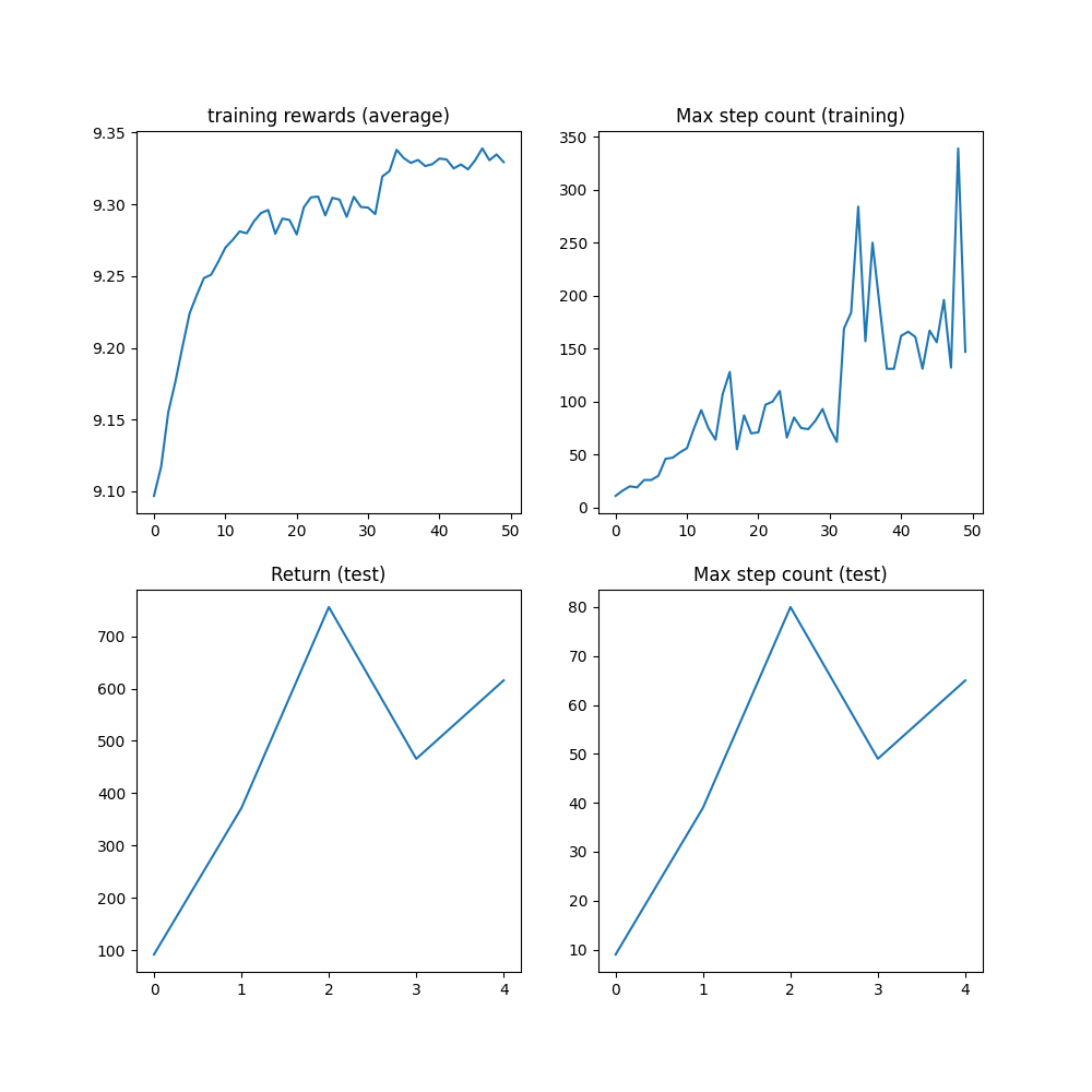
結果¶

在達到 1M 步上限之前，該演算法應已達到 1000 步的最大步數，這是軌跡被截斷之前的最大步數。

plt.figure(figsize=(10, 10))
plt.subplot(2, 2, 1)
plt.plot(logs["reward"])
plt.title("training rewards (average)")
plt.subplot(2, 2, 2)
plt.plot(logs["step_count"])
plt.title("Max step count (training)")
plt.subplot(2, 2, 3)
plt.plot(logs["eval reward (sum)"])
plt.title("Return (test)")
plt.subplot(2, 2, 4)
plt.plot(logs["eval step_count"])
plt.title("Max step count (test)")
plt.show()

training rewards (average), Max step count (training), Return (test), Max step count (test)

結論和下一步¶

在本教學中，我們學到了：

如何使用 torchrl 建立和自訂環境；
如何編寫模型和損失函數；
如何設定典型的訓練迴圈。

如果您想對本教學進行更多實驗，可以應用以下修改：

從效率的角度來看，我們可以並行運行多個模擬以加速資料收集。請查看 ParallelEnv 以獲取更多資訊。
從日誌記錄的角度來看，可以在請求渲染後，將 torchrl.record.VideoRecorder 轉換添加到環境中，以獲得倒立擺動作的可視化渲染。請查看 torchrl.record 以了解更多資訊。

腳本的總運行時間： (3 分鐘 10.450 秒)

由 Sphinx-Gallery 產生的圖庫