(可選) 從 PyTorch 匯出模型至 ONNX 並使用 ONNX Runtime 執行

建立於：2019 年 7 月 17 日 | 最後更新：2024 年 7 月 17 日 | 最後驗證：2024 年 11 月 05 日

注意

從 PyTorch 2.1 開始，ONNX Exporter 有兩個版本。

• torch.onnx.dynamo_export 是最新的 (仍在 beta) Exporter，基於 PyTorch 2.0 發佈的 TorchDynamo 技術。

• torch.onnx.export 基於 TorchScript 後端，自 PyTorch 1.2.0 以來可用。

在本教學中，我們將描述如何使用 TorchScript torch.onnx.export ONNX Exporter 將 PyTorch 中定義的模型轉換為 ONNX 格式。

匯出的模型將使用 ONNX Runtime 執行。ONNX Runtime 是一個以效能為重點的 ONNX 模型引擎，可在多個平台和硬體 (Windows、Linux 和 Mac，以及 CPU 和 GPU) 上有效率地進行推論。 ONNX Runtime 已證明可以顯著提高多個模型的效能，如此處所述

對於本教學，您需要安裝 ONNX 和 ONNX Runtime。您可以使用以下命令取得 ONNX 和 ONNX Runtime 的二進位檔：

%%bash
pip install onnx onnxruntime

ONNX Runtime 建議使用 PyTorch 的最新穩定版 Runtime。

# Some standard imports
import numpy as np

from torch import nn
import torch.utils.model_zoo as model_zoo
import torch.onnx

超解析度是一種提高圖像、影片解析度的方法，廣泛用於圖像處理或影片編輯。在本教學中，我們將使用一個小的超解析度模型。

首先，讓我們在 PyTorch 中建立一個 SuperResolution 模型。該模型使用 “Real-Time Single Image and Video Super-Resolution Using an Efficient Sub-Pixel Convolutional Neural Network” - Shi et al 中描述的有效率的子像素卷積層，透過 upscale 因子提高圖像的解析度。該模型期望圖像的 YCbCr 的 Y 分量作為輸入，並輸出超解析度中 upscale 的 Y 分量。

該模型直接來自 PyTorch 的範例，沒有經過修改

# Super Resolution model definition in PyTorch
import torch.nn as nn
import torch.nn.init as init


class SuperResolutionNet(nn.Module):
    def __init__(self, upscale_factor, inplace=False):
        super(SuperResolutionNet, self).__init__()

        self.relu = nn.ReLU(inplace=inplace)
        self.conv1 = nn.Conv2d(1, 64, (5, 5), (1, 1), (2, 2))
        self.conv2 = nn.Conv2d(64, 64, (3, 3), (1, 1), (1, 1))
        self.conv3 = nn.Conv2d(64, 32, (3, 3), (1, 1), (1, 1))
        self.conv4 = nn.Conv2d(32, upscale_factor ** 2, (3, 3), (1, 1), (1, 1))
        self.pixel_shuffle = nn.PixelShuffle(upscale_factor)

        self._initialize_weights()

    def forward(self, x):
        x = self.relu(self.conv1(x))
        x = self.relu(self.conv2(x))
        x = self.relu(self.conv3(x))
        x = self.pixel_shuffle(self.conv4(x))
        return x

    def _initialize_weights(self):
        init.orthogonal_(self.conv1.weight, init.calculate_gain('relu'))
        init.orthogonal_(self.conv2.weight, init.calculate_gain('relu'))
        init.orthogonal_(self.conv3.weight, init.calculate_gain('relu'))
        init.orthogonal_(self.conv4.weight)

# Create the super-resolution model by using the above model definition.
torch_model = SuperResolutionNet(upscale_factor=3)

通常，您現在會訓練這個模型；但是，在本教學中，我們將改為下載一些預先訓練的權重。請注意，此模型並未經過充分訓練以獲得良好的準確性，在此僅用於演示目的。

在匯出模型之前，呼叫 torch_model.eval() 或 torch_model.train(False) 將模型轉換為推論模式非常重要。這是必需的，因為像 dropout 或 batchnorm 這樣的運算符在推論和訓練模式下的行為不同。

# Load pretrained model weights
model_url = 'https://s3.amazonaws.com/pytorch/test_data/export/superres_epoch100-44c6958e.pth'
batch_size = 64    # just a random number

# Initialize model with the pretrained weights
map_location = lambda storage, loc: storage
if torch.cuda.is_available():
    map_location = None
torch_model.load_state_dict(model_zoo.load_url(model_url, map_location=map_location))

# set the model to inference mode
torch_model.eval()

在 PyTorch 中匯出模型可透過追蹤 (tracing) 或腳本 (scripting) 進行。本教學將以追蹤方式匯出的模型為例。要匯出模型，我們呼叫 torch.onnx.export() 函數。這將執行模型，記錄運算輸出時所使用的運算子軌跡。因為 export 會執行模型，所以我們需要提供輸入張量 x。其中的值可以是隨機的，只要類型和大小正確即可。請注意，除非指定為動態軸，否則輸入大小將在匯出的 ONNX 圖形中針對所有輸入維度固定。在本範例中，我們以 batch_size 為 1 的輸入匯出模型，然後在 torch.onnx.export() 中的 dynamic_axes 參數中將第一維度指定為動態。因此，匯出的模型將接受大小為 [batch_size, 1, 224, 224] 的輸入，其中 batch_size 可以是變數。

要了解有關 PyTorch 匯出介面的更多詳細資訊，請查看 torch.onnx 文件。

# Input to the model
x = torch.randn(batch_size, 1, 224, 224, requires_grad=True)
torch_out = torch_model(x)

# Export the model
torch.onnx.export(torch_model,               # model being run
                  x,                         # model input (or a tuple for multiple inputs)
                  "super_resolution.onnx",   # where to save the model (can be a file or file-like object)
                  export_params=True,        # store the trained parameter weights inside the model file
                  opset_version=10,          # the ONNX version to export the model to
                  do_constant_folding=True,  # whether to execute constant folding for optimization
                  input_names = ['input'],   # the model's input names
                  output_names = ['output'], # the model's output names
                  dynamic_axes={'input' : {0 : 'batch_size'},    # variable length axes
                                'output' : {0 : 'batch_size'}})

我們也計算了 torch_out，即模型執行後的輸出，我們將使用它來驗證我們匯出的模型在 ONNX Runtime 中執行時計算的值是否相同。

但在使用 ONNX Runtime 驗證模型的輸出之前，我們將使用 ONNX API 檢查 ONNX 模型。首先，onnx.load("super_resolution.onnx") 將載入已儲存的模型，並輸出一個 onnx.ModelProto 結構 (用於捆綁 ML 模型的最上層檔案/容器格式。如需更多資訊，請參閱 onnx.proto 文件)。然後，onnx.checker.check_model(onnx_model) 將驗證模型的結構，並確認模型具有有效的綱要。ONNX 圖形的有效性是透過檢查模型的版本、圖形的結構，以及節點及其輸入和輸出來驗證的。

import onnx

onnx_model = onnx.load("super_resolution.onnx")
onnx.checker.check_model(onnx_model)

現在讓我們使用 ONNX Runtime 的 Python API 計算輸出。這部分通常可以在單獨的進程或在另一台機器上完成，但我們將在同一個進程中繼續進行，以便我們可以驗證 ONNX Runtime 和 PyTorch 是否為網路計算相同的值。

為了使用 ONNX Runtime 執行模型，我們需要使用選定的配置參數 (這裡我們使用預設配置) 為模型建立一個推論會話。建立會話後，我們使用 run() API 評估模型。此呼叫的輸出是一個列表，其中包含 ONNX Runtime 計算的模型輸出。

import onnxruntime

ort_session = onnxruntime.InferenceSession("super_resolution.onnx", providers=["CPUExecutionProvider"])

def to_numpy(tensor):
    return tensor.detach().cpu().numpy() if tensor.requires_grad else tensor.cpu().numpy()

# compute ONNX Runtime output prediction
ort_inputs = {ort_session.get_inputs()[0].name: to_numpy(x)}
ort_outs = ort_session.run(None, ort_inputs)

# compare ONNX Runtime and PyTorch results
np.testing.assert_allclose(to_numpy(torch_out), ort_outs[0], rtol=1e-03, atol=1e-05)

print("Exported model has been tested with ONNXRuntime, and the result looks good!")

我們應該看到 PyTorch 和 ONNX Runtime 執行的輸出在數值上與給定的精度 (rtol=1e-03 和 atol=1e-05) 相符。順帶一提，如果它們不匹配，則 ONNX 匯出器存在問題，請在這種情況下與我們聯繫。

模型之間的時序比較

由於 ONNX 模型針對推論速度進行了最佳化，因此在 ONNX 模型而不是原生 pytorch 模型上執行相同的數據應該會使效能提升高達 2 倍。批次大小越大，效能提升越明顯。

import time

x = torch.randn(batch_size, 1, 224, 224, requires_grad=True)

start = time.time()
torch_out = torch_model(x)
end = time.time()
print(f"Inference of Pytorch model used {end - start} seconds")

ort_inputs = {ort_session.get_inputs()[0].name: to_numpy(x)}
start = time.time()
ort_outs = ort_session.run(None, ort_inputs)
end = time.time()
print(f"Inference of ONNX model used {end - start} seconds")

使用 ONNX Runtime 在圖像上執行模型

到目前為止，我們已經從 PyTorch 匯出了一個模型，並展示了如何在 ONNX Runtime 中載入和執行它，並以虛擬張量作為輸入。

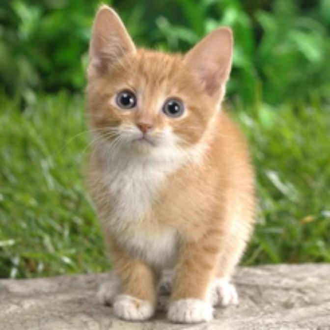
在本教學中，我們將使用一張廣泛使用的著名貓圖片，如下所示

首先，讓我們載入圖像，並使用標準 PIL python 庫對其進行預處理。請注意，此預處理是訓練/測試神經網路數據的標準實務。

我們首先調整圖像大小以適合模型輸入的大小 (224x224)。然後，我們將圖像分割為 Y、Cb 和 Cr 分量。這些分量代表灰階圖像 (Y)，以及藍色差 (Cb) 和紅色差 (Cr) 色度分量。由於 Y 分量對人眼更敏感，因此我們對此分量感興趣，我們將對其進行轉換。提取 Y 分量後，我們將其轉換為張量，這將是我們模型的輸入。

from PIL import Image
import torchvision.transforms as transforms

img = Image.open("./_static/img/cat.jpg")

resize = transforms.Resize([224, 224])
img = resize(img)

img_ycbcr = img.convert('YCbCr')
img_y, img_cb, img_cr = img_ycbcr.split()

to_tensor = transforms.ToTensor()
img_y = to_tensor(img_y)
img_y.unsqueeze_(0)

現在，作為下一步，讓我們取得代表灰階調整大小的貓圖像的張量，並如先前所述在 ONNX Runtime 中執行超解析度模型。

ort_inputs = {ort_session.get_inputs()[0].name: to_numpy(img_y)}
ort_outs = ort_session.run(None, ort_inputs)
img_out_y = ort_outs[0]

此時，模型的輸出是一個張量。現在，我們將處理模型的輸出，以從輸出張量建構回最終輸出圖像，並儲存圖像。後處理步驟已從 PyTorch 超解析度模型的實作中採用 here。

img_out_y = Image.fromarray(np.uint8((img_out_y[0] * 255.0).clip(0, 255)[0]), mode='L')

# get the output image follow post-processing step from PyTorch implementation
final_img = Image.merge(
    "YCbCr", [
        img_out_y,
        img_cb.resize(img_out_y.size, Image.BICUBIC),
        img_cr.resize(img_out_y.size, Image.BICUBIC),
    ]).convert("RGB")

# Save the image, we will compare this with the output image from mobile device
final_img.save("./_static/img/cat_superres_with_ort.jpg")

# Save resized original image (without super-resolution)
img = transforms.Resize([img_out_y.size[0], img_out_y.size[1]])(img)
img.save("cat_resized.jpg")

以下是兩張圖片之間的比較

低解析度圖像

超解析度後的圖像

ONNX Runtime 是一個跨平台引擎，您可以在多個平台以及 CPU 和 GPU 上執行它。

ONNX Runtime 也可以使用 Azure Machine Learning Services 部署到雲端以進行模型推論。更多資訊 here。

有關 ONNX Runtime 效能的更多資訊 here。

有關 ONNX Runtime 的更多資訊 here。