強化學習 (DQN) 教學

建立於：2017 年 3 月 24 日 | 最後更新：2024 年 6 月 18 日 | 最後驗證：2024 年 11 月 05 日

作者: Adam Paszke

Mark Towers

本教學展示如何使用 PyTorch 在來自 Gymnasium 的 CartPole-v1 任務上訓練深度 Q 學習 (DQN) 代理。

您可能會覺得閱讀原始的 深度 Q 學習 (DQN) 論文很有幫助

任務

代理必須在兩個動作之間做出決定 - 向左或向右移動推車 - 以便連接到推車的桿保持直立。您可以在 Gymnasium 的網站上找到有關環境和其他更具挑戰性環境的更多資訊。

CartPole

當代理觀察環境的目前狀態並選擇一個動作時，環境會轉換到一個新的狀態，並且還會返回一個獎勵，指示該動作的後果。在此任務中，每次遞增的時間步都會獲得 +1 的獎勵，如果桿子倒下太遠或推車移動超過距離中心 2.4 個單位的距離，環境就會終止。這表示效能較佳的情境將會運行更長時間，累積更大的回報。

CartPole 任務的設計方式是代理的輸入是 4 個代表環境狀態 (位置、速度等) 的實數值。我們不經過任何縮放就取得這 4 個輸入，並將它們傳遞到一個具有 2 個輸出的小型全連接網路，每個動作一個輸出。訓練網路來預測每個動作的預期值，給定輸入狀態。然後選擇具有最高預期值的動作。

套件

首先，讓我們匯入所需的套件。首先，我們需要 gymnasium 來進行環境，使用 pip 安裝。這是原始 OpenAI Gym 專案的一個分支，自 Gym v0.19 以來由同一團隊維護。如果您在 Google Colab 中執行此操作，請執行

%%bash
pip3 install gymnasium[classic_control]

我們還將使用 PyTorch 中的以下內容

• 神經網路 (torch.nn)

• 最佳化 (torch.optim)

• 自動微分 (torch.autograd)

import gymnasium as gym
import math
import random
import matplotlib
import matplotlib.pyplot as plt
from collections import namedtuple, deque
from itertools import count

import torch
import torch.nn as nn
import torch.optim as optim
import torch.nn.functional as F

env = gym.make("CartPole-v1")

# set up matplotlib
is_ipython = 'inline' in matplotlib.get_backend()
if is_ipython:
    from IPython import display

plt.ion()

# if GPU is to be used
device = torch.device(
    "cuda" if torch.cuda.is_available() else
    "mps" if torch.backends.mps.is_available() else
    "cpu"
)

重播記憶體

我們將使用經驗重播記憶體來訓練我們的 DQN。它會儲存代理觀察到的轉換，讓我們可以在稍後重複使用此資料。透過從中隨機取樣，建立批次的轉換會被去相關。已經證明，這可以大大穩定和改善 DQN 訓練程序。

為此，我們需要兩個類別

• Transition - 一個 named tuple，代表我們環境中的單一轉換。它基本上將 (狀態、動作) 配對對應到它們的 (next_state、reward) 結果，其中狀態是稍後描述的螢幕差異影像。

• ReplayMemory - 一個有界大小的循環緩衝區，用於保存最近觀察到的轉換。它還實作一個 .sample() 方法，用於選擇用於訓練的隨機轉換批次。

Transition = namedtuple('Transition',
                        ('state', 'action', 'next_state', 'reward'))


class ReplayMemory(object):

    def __init__(self, capacity):
        self.memory = deque([], maxlen=capacity)

    def push(self, *args):
        """Save a transition"""
        self.memory.append(Transition(*args))

    def sample(self, batch_size):
        return random.sample(self.memory, batch_size)

    def __len__(self):
        return len(self.memory)

現在，讓我們定義我們的模型。但首先，讓我們快速回顧一下 DQN 是什麼。

DQN 演算法

我們的環境是確定性的，因此為了簡單起見，這裡呈現的所有方程式也都是以確定性的方式表述的。在強化學習文獻中，它們也會包含環境中隨機轉換的期望值。

我們的目標是訓練一個策略，嘗試最大化折扣的累積獎勵 \(R_{t_0} = \sum_{t=t_0}^{\infty} \gamma^{t - t_0} r_t\)，其中 \(R_{t_0}\) 也稱為回報。折扣 \(\gamma\) 應該是介於 \(0\) 和 \(1\) 之間的常數，以確保總和收斂。較低的 \(\gamma\) 使得來自不確定的遙遠未來的獎勵對於我們的代理來說，不如對近期獎勵重要，因為代理可以對這些獎勵相當有信心。它還鼓勵代理收集時間上較近的獎勵，而不是在未來時間上較遠的等效獎勵。

Q 學習背後的主要思想是，如果我們有一個函數 \(Q^*: State \times Action \rightarrow \mathbb{R}\)，可以告訴我們如果我們在給定的狀態下採取一個動作，我們的回報會是多少，那麼我們可以很容易地建構一個最大化我們獎勵的策略

\[\pi^*(s) = \arg\!\max_a \ Q^*(s, a) \]

但是，我們並不知道關於世界的所有事情，因此我們無法存取 \(Q^*\)。但是，由於神經網路是通用函數逼近器，我們可以簡單地建立一個並訓練它，使其類似於 \(Q^*\)。

對於我們的訓練更新規則，我們將使用一個事實，即某些策略的每個 \(Q\) 函數都遵循貝爾曼方程式

\[Q^{\pi}(s, a) = r + \gamma Q^{\pi}(s', \pi(s')) \]

等式兩邊的差異稱為時間差分誤差，\(\delta\)

\[\delta = Q(s, a) - (r + \gamma \max_a' Q(s', a)) \]

為了最小化這個誤差，我們將使用 Huber 損失。當誤差很小時，Huber 損失的作用類似於均方誤差；但當誤差很大時，其作用類似於平均絕對誤差 - 這使得它在 \(Q\) 的估計值非常noisy時，對於離群值更加穩健。我們針對從重播記憶體中取樣的一批轉換 \(B\) 來計算這個損失

\[\mathcal{L} = \frac{1}{|B|}\sum_{(s, a, s', r) \ \in \ B} \mathcal{L}(\delta)\]

\[\text{其中} \quad \mathcal{L}(\delta) = \begin{cases} \frac{1}{2}{\delta^2} & \text{如果 } |\delta| \le 1, \\ |\delta| - \frac{1}{2} & \text{其他情況.} \end{cases}\]

Q 網路

我們的模型將會是一個前饋神經網路，它接收目前螢幕區塊和先前螢幕區塊之間的差異。它有兩個輸出，分別代表 \(Q(s, \mathrm{left})\) 和 \(Q(s, \mathrm{right})\)（其中 \(s\) 是網路的輸入）。實際上，網路正在嘗試預測在給定目前輸入的情況下，採取每個動作的預期回報。

class DQN(nn.Module):

    def __init__(self, n_observations, n_actions):
        super(DQN, self).__init__()
        self.layer1 = nn.Linear(n_observations, 128)
        self.layer2 = nn.Linear(128, 128)
        self.layer3 = nn.Linear(128, n_actions)

    # Called with either one element to determine next action, or a batch
    # during optimization. Returns tensor([[left0exp,right0exp]...]).
    def forward(self, x):
        x = F.relu(self.layer1(x))
        x = F.relu(self.layer2(x))
        return self.layer3(x)

訓練

超參數與工具

此儲存格會實例化我們的模型及其優化器，並定義一些工具

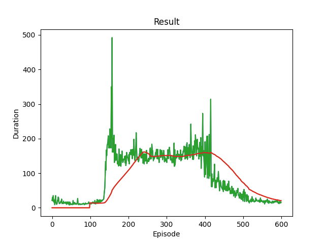
• select_action - 將根據 epsilon 貪婪策略選擇動作。簡單來說，我們有時會使用我們的模型來選擇動作，有時我們會直接均勻地取樣一個動作。選擇隨機動作的機率將從 EPS_START 開始，並以指數方式衰減到 EPS_END。EPS_DECAY 控制衰減率。

• plot_durations - 一個用於繪製 episodes 持續時間的輔助函數，以及過去 100 個 episodes 的平均值（官方評估中使用的度量）。該圖將位於包含主要訓練迴圈的儲存格下方，並將在每個 episode 之後更新。

# BATCH_SIZE is the number of transitions sampled from the replay buffer
# GAMMA is the discount factor as mentioned in the previous section
# EPS_START is the starting value of epsilon
# EPS_END is the final value of epsilon
# EPS_DECAY controls the rate of exponential decay of epsilon, higher means a slower decay
# TAU is the update rate of the target network
# LR is the learning rate of the ``AdamW`` optimizer
BATCH_SIZE = 128
GAMMA = 0.99
EPS_START = 0.9
EPS_END = 0.05
EPS_DECAY = 1000
TAU = 0.005
LR = 1e-4

# Get number of actions from gym action space
n_actions = env.action_space.n
# Get the number of state observations
state, info = env.reset()
n_observations = len(state)

policy_net = DQN(n_observations, n_actions).to(device)
target_net = DQN(n_observations, n_actions).to(device)
target_net.load_state_dict(policy_net.state_dict())

optimizer = optim.AdamW(policy_net.parameters(), lr=LR, amsgrad=True)
memory = ReplayMemory(10000)


steps_done = 0


def select_action(state):
    global steps_done
    sample = random.random()
    eps_threshold = EPS_END + (EPS_START - EPS_END) * \
        math.exp(-1. * steps_done / EPS_DECAY)
    steps_done += 1
    if sample > eps_threshold:
        with torch.no_grad():
            # t.max(1) will return the largest column value of each row.
            # second column on max result is index of where max element was
            # found, so we pick action with the larger expected reward.
            return policy_net(state).max(1).indices.view(1, 1)
    else:
        return torch.tensor([[env.action_space.sample()]], device=device, dtype=torch.long)


episode_durations = []


def plot_durations(show_result=False):
    plt.figure(1)
    durations_t = torch.tensor(episode_durations, dtype=torch.float)
    if show_result:
        plt.title('Result')
    else:
        plt.clf()
        plt.title('Training...')
    plt.xlabel('Episode')
    plt.ylabel('Duration')
    plt.plot(durations_t.numpy())
    # Take 100 episode averages and plot them too
    if len(durations_t) >= 100:
        means = durations_t.unfold(0, 100, 1).mean(1).view(-1)
        means = torch.cat((torch.zeros(99), means))
        plt.plot(means.numpy())

    plt.pause(0.001)  # pause a bit so that plots are updated
    if is_ipython:
        if not show_result:
            display.display(plt.gcf())
            display.clear_output(wait=True)
        else:
            display.display(plt.gcf())

訓練迴圈

最後，這是訓練我們模型的程式碼。

在這裡，您可以找到一個 optimize_model 函數，它執行優化的單一步驟。它首先取樣一個批次，將所有張量連接到一個單一張量中，計算 \(Q(s_t, a_t)\) 和 \(V(s_{t+1}) = \max_a Q(s_{t+1}, a)\)，並將它們組合成我們的損失。根據定義，如果 \(s\) 是一個終端狀態，我們將 \(V(s) = 0\) 設置為 0。我們也使用目標網路來計算 \(V(s_{t+1})\) 以增加穩定性。目標網路在每個步驟都會使用由超參數 TAU 控制的 軟更新 來更新，該參數先前已定義。

def optimize_model():
    if len(memory) < BATCH_SIZE:
        return
    transitions = memory.sample(BATCH_SIZE)
    # Transpose the batch (see https://stackoverflow.com/a/19343/3343043 for
    # detailed explanation). This converts batch-array of Transitions
    # to Transition of batch-arrays.
    batch = Transition(*zip(*transitions))

    # Compute a mask of non-final states and concatenate the batch elements
    # (a final state would've been the one after which simulation ended)
    non_final_mask = torch.tensor(tuple(map(lambda s: s is not None,
                                          batch.next_state)), device=device, dtype=torch.bool)
    non_final_next_states = torch.cat([s for s in batch.next_state
                                                if s is not None])
    state_batch = torch.cat(batch.state)
    action_batch = torch.cat(batch.action)
    reward_batch = torch.cat(batch.reward)

    # Compute Q(s_t, a) - the model computes Q(s_t), then we select the
    # columns of actions taken. These are the actions which would've been taken
    # for each batch state according to policy_net
    state_action_values = policy_net(state_batch).gather(1, action_batch)

    # Compute V(s_{t+1}) for all next states.
    # Expected values of actions for non_final_next_states are computed based
    # on the "older" target_net; selecting their best reward with max(1).values
    # This is merged based on the mask, such that we'll have either the expected
    # state value or 0 in case the state was final.
    next_state_values = torch.zeros(BATCH_SIZE, device=device)
    with torch.no_grad():
        next_state_values[non_final_mask] = target_net(non_final_next_states).max(1).values
    # Compute the expected Q values
    expected_state_action_values = (next_state_values * GAMMA) + reward_batch

    # Compute Huber loss
    criterion = nn.SmoothL1Loss()
    loss = criterion(state_action_values, expected_state_action_values.unsqueeze(1))

    # Optimize the model
    optimizer.zero_grad()
    loss.backward()
    # In-place gradient clipping
    torch.nn.utils.clip_grad_value_(policy_net.parameters(), 100)
    optimizer.step()

在下方，您可以找到主要訓練迴圈。一開始，我們重置環境並獲得初始的 state 張量。然後，我們取樣一個動作，執行它，觀察下一個狀態和獎勵（始終為 1），並優化我們的模型一次。當 episode 結束時（我們的模型失敗），我們重新開始迴圈。

下方，如果可以使用 GPU，num_episodes 會設置為 600，否則會排定 50 個 episodes，以避免訓練時間過長。但是，50 個 episodes 不足以觀察到 CartPole 的良好效能。您應該會看到模型在 600 個訓練 episodes 內不斷地達到 500 步。訓練 RL agents 可能是一個 noisy 的過程，因此如果沒有觀察到收斂，重新開始訓練可以產生更好的結果。

if torch.cuda.is_available() or torch.backends.mps.is_available():
    num_episodes = 600
else:
    num_episodes = 50

for i_episode in range(num_episodes):
    # Initialize the environment and get its state
    state, info = env.reset()
    state = torch.tensor(state, dtype=torch.float32, device=device).unsqueeze(0)
    for t in count():
        action = select_action(state)
        observation, reward, terminated, truncated, _ = env.step(action.item())
        reward = torch.tensor([reward], device=device)
        done = terminated or truncated

        if terminated:
            next_state = None
        else:
            next_state = torch.tensor(observation, dtype=torch.float32, device=device).unsqueeze(0)

        # Store the transition in memory
        memory.push(state, action, next_state, reward)

        # Move to the next state
        state = next_state

        # Perform one step of the optimization (on the policy network)
        optimize_model()

        # Soft update of the target network's weights
        # θ′ ← τ θ + (1 −τ )θ′
        target_net_state_dict = target_net.state_dict()
        policy_net_state_dict = policy_net.state_dict()
        for key in policy_net_state_dict:
            target_net_state_dict[key] = policy_net_state_dict[key]*TAU + target_net_state_dict[key]*(1-TAU)
        target_net.load_state_dict(target_net_state_dict)

        if done:
            episode_durations.append(t + 1)
            plot_durations()
            break

print('Complete')
plot_durations(show_result=True)
plt.ioff()
plt.show()

/usr/local/lib/python3.10/dist-packages/gymnasium/utils/passive_env_checker.py:249: DeprecationWarning:

`np.bool8` is a deprecated alias for `np.bool_`.  (Deprecated NumPy 1.24)

Complete

這是說明整體結果資料流程的圖表。

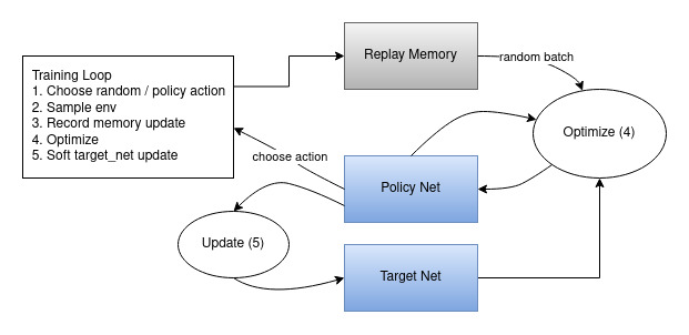
動作可以隨機選擇，也可以根據策略選擇，從 gym 環境中獲取下一個步驟樣本。我們將結果記錄在重播記憶體中，並在每次迭代時執行優化步驟。優化從重播記憶體中選擇一個隨機批次來訓練新策略。「較舊的」target_net 也用於優化中，以計算預期的 Q 值。它的權重會在每個步驟執行軟更新。