知識蒸餾教學

建立於：2023 年 8 月 22 日 | 最後更新：2025 年 1 月 24 日 | 最後驗證：2024 年 11 月 05 日

作者: Alexandros Chariton

知識蒸餾是一種技術，可以將知識從大型、計算成本高的模型轉移到較小的模型，而不會失去有效性。 這允許在功能較弱的硬體上進行部署，從而使評估更快且更有效率。

在本教學中，我們將執行一系列實驗，重點在使用更強大的網路作為教師的情況下，提高輕量級神經網路的準確性。 輕量級網路的計算成本和速度將不受影響，我們的干預僅集中在其權重上，而不是在其正向傳播上。 這種技術的應用可以在無人機或手機等裝置中找到。 在本教學中，我們不使用任何外部套件，因為我們需要的東西都可以在 torch 和 torchvision 中找到。

在本教學中，你將學習

• 如何修改模型類別以提取隱藏表示並將其用於進一步的計算

• 如何修改 PyTorch 中的常規訓練迴圈，以在例如用於分類的交叉熵之上包含額外的損失

• 如何透過使用更複雜的模型作為教師來提高輕量級模型的效能

先決條件

• 1 個 GPU，4GB 記憶體

• PyTorch v2.0 或更新版本

• CIFAR-10 資料集（由腳本下載並儲存在名為 /data 的目錄中）

import torch
import torch.nn as nn
import torch.optim as optim
import torchvision.transforms as transforms
import torchvision.datasets as datasets

# Check if the current `accelerator <https://pytorch.dev.org.tw/docs/stable/torch.html#accelerators>`__
# is available, and if not, use the CPU
device = torch.accelerator.current_accelerator().type if torch.accelerator.is_available() else "cpu"
print(f"Using {device} device")

Using cuda device

載入 CIFAR-10

CIFAR-10 是一個流行的圖像資料集，包含十個類別。 我們的目標是預測每個輸入圖像的以下類別之一。

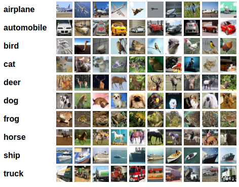
CIFAR-10 圖像範例

輸入圖像為 RGB，因此它們有 3 個通道，並且是 32x32 像素。 基本上，每個圖像都由 3 x 32 x 32 = 3072 個範圍從 0 到 255 的數字描述。 神經網路中的常見做法是正規化輸入，這樣做的原因有很多，包括避免常用啟動函數中的飽和並提高數值穩定性。 我們的正規化過程包括減去均值並沿每個通道除以標準差。 張量“mean=[0.485, 0.456, 0.406]”和“std=[0.229, 0.224, 0.225]”已經計算過了，它們代表 CIFAR-10 預定義子集中每個通道的均值和標準差，該子集旨在成為訓練集。 請注意，我們如何將這些值也用於測試集，而無需從頭重新計算均值和標準差。 這是因為該網路是在透過減去和除以上面的數字產生的特徵上訓練的，我們希望保持一致性。 此外，在現實生活中，我們將無法計算測試集的均值和標準差，因為根據我們的假設，此資料在當時將無法存取。

作為最後一點，我們通常將此保留集稱為驗證集，並且在優化模型在驗證集上的效能後，我們使用一個單獨的集合，稱為測試集。 這樣做是為了避免根據單一指標的貪婪和有偏差的優化來選擇模型。

# Below we are preprocessing data for CIFAR-10. We use an arbitrary batch size of 128.
transforms_cifar = transforms.Compose([
    transforms.ToTensor(),
    transforms.Normalize(mean=[0.485, 0.456, 0.406], std=[0.229, 0.224, 0.225]),
])

# Loading the CIFAR-10 dataset:
train_dataset = datasets.CIFAR10(root='./data', train=True, download=True, transform=transforms_cifar)
test_dataset = datasets.CIFAR10(root='./data', train=False, download=True, transform=transforms_cifar)

  0%|          | 0.00/170M [00:00<?, ?B/s]
  0%|          | 754k/170M [00:00<00:22, 7.53MB/s]
  4%|4         | 7.50M/170M [00:00<00:03, 42.8MB/s]
 10%|9         | 17.0M/170M [00:00<00:02, 66.2MB/s]
 16%|#5        | 26.7M/170M [00:00<00:01, 78.4MB/s]
 22%|##1       | 36.7M/170M [00:00<00:01, 86.2MB/s]
 27%|##7       | 46.8M/170M [00:00<00:01, 90.9MB/s]
 33%|###3      | 56.7M/170M [00:00<00:01, 93.6MB/s]
 39%|###8      | 66.5M/170M [00:00<00:01, 94.7MB/s]
 45%|####4     | 76.2M/170M [00:00<00:00, 95.3MB/s]
 51%|#####     | 86.4M/170M [00:01<00:00, 97.2MB/s]
 57%|#####7    | 97.4M/170M [00:01<00:00, 101MB/s]
 64%|######3   | 108M/170M [00:01<00:00, 104MB/s]
 70%|######9   | 119M/170M [00:01<00:00, 104MB/s]
 76%|#######5  | 129M/170M [00:01<00:00, 96.3MB/s]
 82%|########1 | 139M/170M [00:01<00:00, 92.1MB/s]
 87%|########7 | 148M/170M [00:01<00:00, 88.2MB/s]
 92%|#########2| 157M/170M [00:01<00:00, 84.1MB/s]
 97%|#########7| 166M/170M [00:01<00:00, 80.4MB/s]
100%|##########| 170M/170M [00:01<00:00, 86.7MB/s]

注意

本節僅適用於對快速結果感興趣的 CPU 使用者。 僅當您對小規模實驗感興趣時才使用此選項。 請記住，使用任何 GPU 程式碼都應該執行得相當快。 僅從訓練/測試資料集中選擇前 num_images_to_keep 個圖像

#from torch.utils.data import Subset
#num_images_to_keep = 2000
#train_dataset = Subset(train_dataset, range(min(num_images_to_keep, 50_000)))
#test_dataset = Subset(test_dataset, range(min(num_images_to_keep, 10_000)))

#Dataloaders
train_loader = torch.utils.data.DataLoader(train_dataset, batch_size=128, shuffle=True, num_workers=2)
test_loader = torch.utils.data.DataLoader(test_dataset, batch_size=128, shuffle=False, num_workers=2)

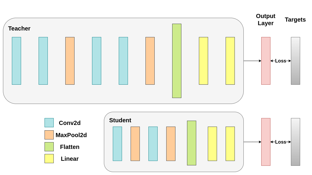
定義模型類別和實用函數

接下來，我們需要定義我們的模型類別。這裡需要設定幾個使用者定義的參數。我們使用兩種不同的架構，並在所有實驗中保持濾波器數量固定，以確保公平的比較。這兩種架構都是卷積神經網路 (CNN)，具有不同數量的卷積層作為特徵提取器，後接一個具有 10 個類別的分類器。學生的濾波器和神經元數量較少。

# Deeper neural network class to be used as teacher:
class DeepNN(nn.Module):
    def __init__(self, num_classes=10):
        super(DeepNN, self).__init__()
        self.features = nn.Sequential(
            nn.Conv2d(3, 128, kernel_size=3, padding=1),
            nn.ReLU(),
            nn.Conv2d(128, 64, kernel_size=3, padding=1),
            nn.ReLU(),
            nn.MaxPool2d(kernel_size=2, stride=2),
            nn.Conv2d(64, 64, kernel_size=3, padding=1),
            nn.ReLU(),
            nn.Conv2d(64, 32, kernel_size=3, padding=1),
            nn.ReLU(),
            nn.MaxPool2d(kernel_size=2, stride=2),
        )
        self.classifier = nn.Sequential(
            nn.Linear(2048, 512),
            nn.ReLU(),
            nn.Dropout(0.1),
            nn.Linear(512, num_classes)
        )

    def forward(self, x):
        x = self.features(x)
        x = torch.flatten(x, 1)
        x = self.classifier(x)
        return x

# Lightweight neural network class to be used as student:
class LightNN(nn.Module):
    def __init__(self, num_classes=10):
        super(LightNN, self).__init__()
        self.features = nn.Sequential(
            nn.Conv2d(3, 16, kernel_size=3, padding=1),
            nn.ReLU(),
            nn.MaxPool2d(kernel_size=2, stride=2),
            nn.Conv2d(16, 16, kernel_size=3, padding=1),
            nn.ReLU(),
            nn.MaxPool2d(kernel_size=2, stride=2),
        )
        self.classifier = nn.Sequential(
            nn.Linear(1024, 256),
            nn.ReLU(),
            nn.Dropout(0.1),
            nn.Linear(256, num_classes)
        )

    def forward(self, x):
        x = self.features(x)
        x = torch.flatten(x, 1)
        x = self.classifier(x)
        return x

我們使用 2 個函數來幫助我們產生和評估原始分類任務的結果。其中一個函數稱為 train，它接受以下參數：

• model：一個模型實例，透過此函數訓練 (更新其權重)。

• train_loader：我們在上面定義了我們的 train_loader，它的工作是將資料饋送到模型中。

• epochs：我們在資料集上循環的次數。

• learning_rate：學習率決定了我們朝收斂方向邁進的步幅大小。過大或過小的步幅都可能造成不利影響。

• device：決定在哪個裝置上執行工作負載。根據可用性，可以是 CPU 或 GPU。

我們的測試函數與之類似，但會使用 test_loader 調用，以從測試集中載入圖像。

使用 Cross-Entropy 訓練兩個網路。學生將被用作基準：

def train(model, train_loader, epochs, learning_rate, device):
    criterion = nn.CrossEntropyLoss()
    optimizer = optim.Adam(model.parameters(), lr=learning_rate)

    model.train()

    for epoch in range(epochs):
        running_loss = 0.0
        for inputs, labels in train_loader:
            # inputs: A collection of batch_size images
            # labels: A vector of dimensionality batch_size with integers denoting class of each image
            inputs, labels = inputs.to(device), labels.to(device)

            optimizer.zero_grad()
            outputs = model(inputs)

            # outputs: Output of the network for the collection of images. A tensor of dimensionality batch_size x num_classes
            # labels: The actual labels of the images. Vector of dimensionality batch_size
            loss = criterion(outputs, labels)
            loss.backward()
            optimizer.step()

            running_loss += loss.item()

        print(f"Epoch {epoch+1}/{epochs}, Loss: {running_loss / len(train_loader)}")

def test(model, test_loader, device):
    model.to(device)
    model.eval()

    correct = 0
    total = 0

    with torch.no_grad():
        for inputs, labels in test_loader:
            inputs, labels = inputs.to(device), labels.to(device)

            outputs = model(inputs)
            _, predicted = torch.max(outputs.data, 1)

            total += labels.size(0)
            correct += (predicted == labels).sum().item()

    accuracy = 100 * correct / total
    print(f"Test Accuracy: {accuracy:.2f}%")
    return accuracy

Cross-entropy 運行

為了可重現性，我們需要設定 torch manual seed。我們使用不同的方法訓練網路，因此為了公平地比較它們，將網路初始化為相同的權重是有意義的。首先使用 cross-entropy 訓練 teacher network

torch.manual_seed(42)
nn_deep = DeepNN(num_classes=10).to(device)
train(nn_deep, train_loader, epochs=10, learning_rate=0.001, device=device)
test_accuracy_deep = test(nn_deep, test_loader, device)

# Instantiate the lightweight network:
torch.manual_seed(42)
nn_light = LightNN(num_classes=10).to(device)

Epoch 1/10, Loss: 1.329837580318646
Epoch 2/10, Loss: 0.8678176775003028
Epoch 3/10, Loss: 0.6815747665932111
Epoch 4/10, Loss: 0.5343365599127377
Epoch 5/10, Loss: 0.41786423847650933
Epoch 6/10, Loss: 0.3018103416847146
Epoch 7/10, Loss: 0.22530553787184493
Epoch 8/10, Loss: 0.16732249605228833
Epoch 9/10, Loss: 0.14114774030911953
Epoch 10/10, Loss: 0.11767084830824066
Test Accuracy: 75.98%

我們實例化另一個輕量級網路模型，以比較它們的效能。反向傳播對權重初始化很敏感，因此我們需要確保這兩個網路具有完全相同的初始化。

torch.manual_seed(42)
new_nn_light = LightNN(num_classes=10).to(device)

為了確保我們建立了第一個網路的副本，我們檢查其第一層的範數。如果匹配，那麼我們可以安全地得出結論，這些網路確實相同。

# Print the norm of the first layer of the initial lightweight model
print("Norm of 1st layer of nn_light:", torch.norm(nn_light.features[0].weight).item())
# Print the norm of the first layer of the new lightweight model
print("Norm of 1st layer of new_nn_light:", torch.norm(new_nn_light.features[0].weight).item())

Norm of 1st layer of nn_light: 2.327361822128296
Norm of 1st layer of new_nn_light: 2.327361822128296

印出每個模型中的參數總數

total_params_deep = "{:,}".format(sum(p.numel() for p in nn_deep.parameters()))
print(f"DeepNN parameters: {total_params_deep}")
total_params_light = "{:,}".format(sum(p.numel() for p in nn_light.parameters()))
print(f"LightNN parameters: {total_params_light}")

DeepNN parameters: 1,186,986
LightNN parameters: 267,738

使用 cross entropy loss 訓練和測試輕量級網路

train(nn_light, train_loader, epochs=10, learning_rate=0.001, device=device)
test_accuracy_light_ce = test(nn_light, test_loader, device)

Epoch 1/10, Loss: 1.4699091780216187
Epoch 2/10, Loss: 1.1620798132303731
Epoch 3/10, Loss: 1.0295765078281198
Epoch 4/10, Loss: 0.9262913492939356
Epoch 5/10, Loss: 0.8496292234991517
Epoch 6/10, Loss: 0.7809841055089556
Epoch 7/10, Loss: 0.7163250502722952
Epoch 8/10, Loss: 0.6582439961030965
Epoch 9/10, Loss: 0.6072786463343579
Epoch 10/10, Loss: 0.5558338365743837
Test Accuracy: 70.65%

正如我們所看到的，根據測試準確性，我們現在可以將將要用作 teacher 的更深層網路與我們假設的 student 的輕量級網路進行比較。到目前為止，我們的 student 尚未干預 teacher，因此此效能是由 student 本身實現的。到目前為止的指標可以在以下幾行中看到

print(f"Teacher accuracy: {test_accuracy_deep:.2f}%")
print(f"Student accuracy: {test_accuracy_light_ce:.2f}%")

Teacher accuracy: 75.98%
Student accuracy: 70.65%

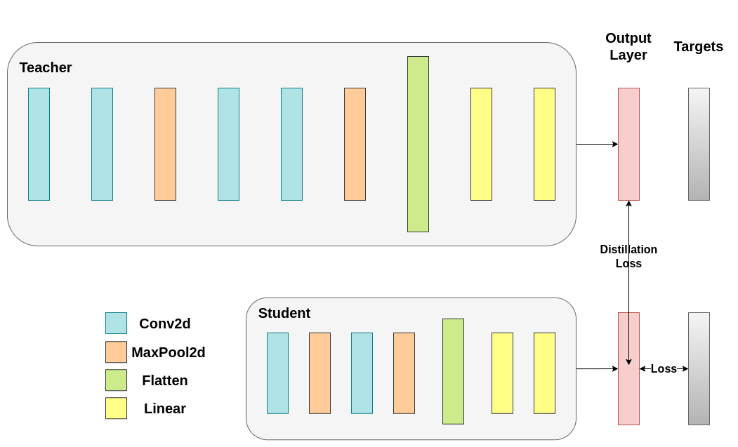
Knowledge distillation 運行

現在讓我們嘗試透過結合 teacher 來提高 student 網路的測試準確性。Knowledge distillation 是一種簡單的技術，可以實現這一目標，基於以下事實：這兩個網路都輸出我們類別上的機率分佈。因此，這兩個網路共享相同數量的輸出神經元。該方法透過將額外的損失納入傳統的 cross entropy loss 中來工作，該損失基於 teacher 網路的 softmax 輸出。假設是，經過適當訓練的 teacher 網路的輸出激活攜帶額外的資訊，student 網路可以在訓練期間利用這些資訊。最初的工作表明，利用 soft targets 中較小機率的比率可以幫助實現深度神經網路的根本目標，即在資料上建立一個相似性結構，其中相似的物件被映射得更近。例如，在 CIFAR-10 中，如果存在輪子，卡車可能會被誤認為是汽車或飛機，但不太可能被誤認為是狗。因此，假設有價值的資訊不僅存在於經過適當訓練的模型的最高預測中，而且存在於整個輸出分佈中是有意義的。然而，僅僅 cross entropy 並不能充分利用此資訊，因為非預測類別的激活往往太小，以至於傳播的梯度無法有意義地改變權重來建構這個理想的向量空間。

當我們繼續定義引入 teacher-student 動態的第一個輔助函數時，我們需要包含一些額外的參數

• T：Temperature 控制輸出分佈的平滑度。較大的 T 導致更平滑的分佈，因此較小的機率會得到更大的提升。

• soft_target_loss_weight：分配給我們即將包含的額外目標的權重。

• ce_loss_weight：分配給 cross-entropy 的權重。調整這些權重會推動網路朝著優化任一目標的方向發展。

Distillation loss 是從網路的 logits 計算得出的。它只會將梯度返回給 student：

def train_knowledge_distillation(teacher, student, train_loader, epochs, learning_rate, T, soft_target_loss_weight, ce_loss_weight, device):
    ce_loss = nn.CrossEntropyLoss()
    optimizer = optim.Adam(student.parameters(), lr=learning_rate)

    teacher.eval()  # Teacher set to evaluation mode
    student.train() # Student to train mode

    for epoch in range(epochs):
        running_loss = 0.0
        for inputs, labels in train_loader:
            inputs, labels = inputs.to(device), labels.to(device)

            optimizer.zero_grad()

            # Forward pass with the teacher model - do not save gradients here as we do not change the teacher's weights
            with torch.no_grad():
                teacher_logits = teacher(inputs)

            # Forward pass with the student model
            student_logits = student(inputs)

            #Soften the student logits by applying softmax first and log() second
            soft_targets = nn.functional.softmax(teacher_logits / T, dim=-1)
            soft_prob = nn.functional.log_softmax(student_logits / T, dim=-1)

            # Calculate the soft targets loss. Scaled by T**2 as suggested by the authors of the paper "Distilling the knowledge in a neural network"
            soft_targets_loss = torch.sum(soft_targets * (soft_targets.log() - soft_prob)) / soft_prob.size()[0] * (T**2)

            # Calculate the true label loss
            label_loss = ce_loss(student_logits, labels)

            # Weighted sum of the two losses
            loss = soft_target_loss_weight * soft_targets_loss + ce_loss_weight * label_loss

            loss.backward()
            optimizer.step()

            running_loss += loss.item()

        print(f"Epoch {epoch+1}/{epochs}, Loss: {running_loss / len(train_loader)}")

# Apply ``train_knowledge_distillation`` with a temperature of 2. Arbitrarily set the weights to 0.75 for CE and 0.25 for distillation loss.
train_knowledge_distillation(teacher=nn_deep, student=new_nn_light, train_loader=train_loader, epochs=10, learning_rate=0.001, T=2, soft_target_loss_weight=0.25, ce_loss_weight=0.75, device=device)
test_accuracy_light_ce_and_kd = test(new_nn_light, test_loader, device)

# Compare the student test accuracy with and without the teacher, after distillation
print(f"Teacher accuracy: {test_accuracy_deep:.2f}%")
print(f"Student accuracy without teacher: {test_accuracy_light_ce:.2f}%")
print(f"Student accuracy with CE + KD: {test_accuracy_light_ce_and_kd:.2f}%")

Epoch 1/10, Loss: 2.3993419985027264
Epoch 2/10, Loss: 1.8816983077837073
Epoch 3/10, Loss: 1.660545251863387
Epoch 4/10, Loss: 1.5025935484015422
Epoch 5/10, Loss: 1.377400197641319
Epoch 6/10, Loss: 1.2623111995894585
Epoch 7/10, Loss: 1.1663545374675175
Epoch 8/10, Loss: 1.0826026804916693
Epoch 9/10, Loss: 1.0063069915527578
Epoch 10/10, Loss: 0.9397082798316351
Test Accuracy: 70.49%
Teacher accuracy: 75.98%
Student accuracy without teacher: 70.65%
Student accuracy with CE + KD: 70.49%

Cosine loss 最小化運行

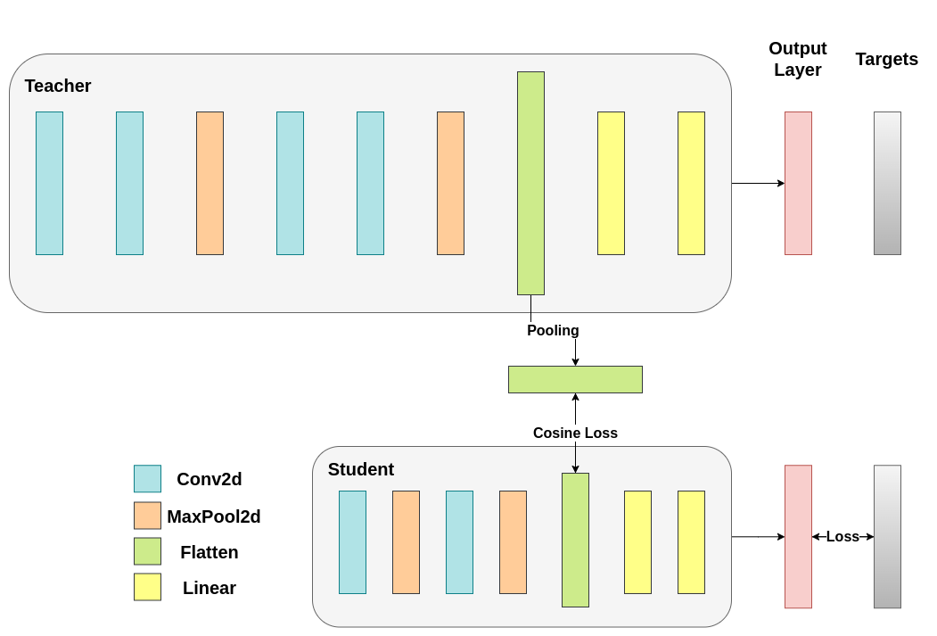
請隨意調整溫度參數，此參數控制 softmax 函數的柔和程度，以及損失係數。在神經網路中，很容易將額外的損失函數加入主要目標中，以實現更好的泛化等目標。讓我們試著為學生加入一個目標，但這次讓我們關注他們的隱藏狀態，而不是輸出層。我們的目標是透過包含一個簡單的損失函數，將老師的表示形式的資訊傳達給學生，此損失函數的最小化意味著隨後傳遞給分類器的展平向量變得更相似，因為損失會減少。當然，老師不會更新其權重，因此最小化僅取決於學生的權重。這種方法背後的原理是，我們假設老師模型具有更好的內部表示形式，如果沒有外部干預，學生不太可能實現此表示形式，因此我們人為地推動學生模仿老師的內部表示形式。然而，這最終是否會對學生有所幫助並不直接，因為推動輕量級網路達到這一點可能是一件好事，假設我們已經找到一個可以提高測試準確性的內部表示形式，但也可能有害，因為網路具有不同的架構，並且學生的學習能力與老師不同。換句話說，沒有理由讓這兩個向量（學生的和老師的）每個分量都匹配。學生可以達到老師的內部表示形式的排列，並且同樣有效。儘管如此，我們仍然可以進行一個快速實驗來確定這種方法的影響。我們將使用 CosineEmbeddingLoss，其公式如下

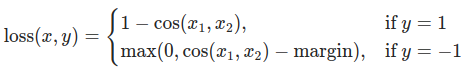
CosineEmbeddingLoss 的公式

顯然，我們首先需要解決一件事。當我們將知識提煉應用於輸出層時，我們提到兩個網路具有相同數量的神經元，等於類別的數量。但是，卷積層之後的層並非如此。在這裡，老師在展平最終卷積層後，擁有的神經元比學生多。我們的損失函數接受兩個相同維度的向量作為輸入，因此我們需要以某種方式匹配它們。我們將透過在老師的卷積層之後包含一個平均池化層來解決這個問題，以減少其維度以匹配學生的維度。

要繼續，我們將修改我們的模型類別，或建立新的類別。現在，前向函數不僅返回網路的 logits，還返回卷積層之後的展平隱藏表示。我們為修改後的老師包含了前面提到的池化。

class ModifiedDeepNNCosine(nn.Module):
    def __init__(self, num_classes=10):
        super(ModifiedDeepNNCosine, self).__init__()
        self.features = nn.Sequential(
            nn.Conv2d(3, 128, kernel_size=3, padding=1),
            nn.ReLU(),
            nn.Conv2d(128, 64, kernel_size=3, padding=1),
            nn.ReLU(),
            nn.MaxPool2d(kernel_size=2, stride=2),
            nn.Conv2d(64, 64, kernel_size=3, padding=1),
            nn.ReLU(),
            nn.Conv2d(64, 32, kernel_size=3, padding=1),
            nn.ReLU(),
            nn.MaxPool2d(kernel_size=2, stride=2),
        )
        self.classifier = nn.Sequential(
            nn.Linear(2048, 512),
            nn.ReLU(),
            nn.Dropout(0.1),
            nn.Linear(512, num_classes)
        )

    def forward(self, x):
        x = self.features(x)
        flattened_conv_output = torch.flatten(x, 1)
        x = self.classifier(flattened_conv_output)
        flattened_conv_output_after_pooling = torch.nn.functional.avg_pool1d(flattened_conv_output, 2)
        return x, flattened_conv_output_after_pooling

# Create a similar student class where we return a tuple. We do not apply pooling after flattening.
class ModifiedLightNNCosine(nn.Module):
    def __init__(self, num_classes=10):
        super(ModifiedLightNNCosine, self).__init__()
        self.features = nn.Sequential(
            nn.Conv2d(3, 16, kernel_size=3, padding=1),
            nn.ReLU(),
            nn.MaxPool2d(kernel_size=2, stride=2),
            nn.Conv2d(16, 16, kernel_size=3, padding=1),
            nn.ReLU(),
            nn.MaxPool2d(kernel_size=2, stride=2),
        )
        self.classifier = nn.Sequential(
            nn.Linear(1024, 256),
            nn.ReLU(),
            nn.Dropout(0.1),
            nn.Linear(256, num_classes)
        )

    def forward(self, x):
        x = self.features(x)
        flattened_conv_output = torch.flatten(x, 1)
        x = self.classifier(flattened_conv_output)
        return x, flattened_conv_output

# We do not have to train the modified deep network from scratch of course, we just load its weights from the trained instance
modified_nn_deep = ModifiedDeepNNCosine(num_classes=10).to(device)
modified_nn_deep.load_state_dict(nn_deep.state_dict())

# Once again ensure the norm of the first layer is the same for both networks
print("Norm of 1st layer for deep_nn:", torch.norm(nn_deep.features[0].weight).item())
print("Norm of 1st layer for modified_deep_nn:", torch.norm(modified_nn_deep.features[0].weight).item())

# Initialize a modified lightweight network with the same seed as our other lightweight instances. This will be trained from scratch to examine the effectiveness of cosine loss minimization.
torch.manual_seed(42)
modified_nn_light = ModifiedLightNNCosine(num_classes=10).to(device)
print("Norm of 1st layer:", torch.norm(modified_nn_light.features[0].weight).item())

Norm of 1st layer for deep_nn: 7.516133785247803
Norm of 1st layer for modified_deep_nn: 7.516133785247803
Norm of 1st layer: 2.327361822128296

自然地，我們需要更改訓練迴圈，因為現在模型返回一個元組 (logits, hidden_representation)。使用範例輸入張量，我們可以列印它們的形狀。

# Create a sample input tensor
sample_input = torch.randn(128, 3, 32, 32).to(device) # Batch size: 128, Filters: 3, Image size: 32x32

# Pass the input through the student
logits, hidden_representation = modified_nn_light(sample_input)

# Print the shapes of the tensors
print("Student logits shape:", logits.shape) # batch_size x total_classes
print("Student hidden representation shape:", hidden_representation.shape) # batch_size x hidden_representation_size

# Pass the input through the teacher
logits, hidden_representation = modified_nn_deep(sample_input)

# Print the shapes of the tensors
print("Teacher logits shape:", logits.shape) # batch_size x total_classes
print("Teacher hidden representation shape:", hidden_representation.shape) # batch_size x hidden_representation_size

Student logits shape: torch.Size([128, 10])
Student hidden representation shape: torch.Size([128, 1024])
Teacher logits shape: torch.Size([128, 10])
Teacher hidden representation shape: torch.Size([128, 1024])

在我們的例子中，hidden_representation_size 是 1024。這是學生最終卷積層的展平特徵圖，正如你所看到的，它是其分類器的輸入。對於老師來說也是 1024，因為我們使用 avg_pool1d 從 2048 使其如此。這裡應用的損失只會影響學生在損失計算之前的權重。換句話說，它不會影響學生的分類器。修改後的訓練迴圈如下

在餘弦損失最小化中，我們希望透過將梯度返回給學生來最大化兩個表示的餘弦相似度：

def train_cosine_loss(teacher, student, train_loader, epochs, learning_rate, hidden_rep_loss_weight, ce_loss_weight, device):
    ce_loss = nn.CrossEntropyLoss()
    cosine_loss = nn.CosineEmbeddingLoss()
    optimizer = optim.Adam(student.parameters(), lr=learning_rate)

    teacher.to(device)
    student.to(device)
    teacher.eval()  # Teacher set to evaluation mode
    student.train() # Student to train mode

    for epoch in range(epochs):
        running_loss = 0.0
        for inputs, labels in train_loader:
            inputs, labels = inputs.to(device), labels.to(device)

            optimizer.zero_grad()

            # Forward pass with the teacher model and keep only the hidden representation
            with torch.no_grad():
                _, teacher_hidden_representation = teacher(inputs)

            # Forward pass with the student model
            student_logits, student_hidden_representation = student(inputs)

            # Calculate the cosine loss. Target is a vector of ones. From the loss formula above we can see that is the case where loss minimization leads to cosine similarity increase.
            hidden_rep_loss = cosine_loss(student_hidden_representation, teacher_hidden_representation, target=torch.ones(inputs.size(0)).to(device))

            # Calculate the true label loss
            label_loss = ce_loss(student_logits, labels)

            # Weighted sum of the two losses
            loss = hidden_rep_loss_weight * hidden_rep_loss + ce_loss_weight * label_loss

            loss.backward()
            optimizer.step()

            running_loss += loss.item()

        print(f"Epoch {epoch+1}/{epochs}, Loss: {running_loss / len(train_loader)}")

我們需要因為相同的原因修改我們的測試函數。在這裡，我們忽略模型返回的隱藏表示。

def test_multiple_outputs(model, test_loader, device):
    model.to(device)
    model.eval()

    correct = 0
    total = 0

    with torch.no_grad():
        for inputs, labels in test_loader:
            inputs, labels = inputs.to(device), labels.to(device)

            outputs, _ = model(inputs) # Disregard the second tensor of the tuple
            _, predicted = torch.max(outputs.data, 1)

            total += labels.size(0)
            correct += (predicted == labels).sum().item()

    accuracy = 100 * correct / total
    print(f"Test Accuracy: {accuracy:.2f}%")
    return accuracy

在這種情況下，我們可以輕鬆地在同一個函數中包含知識提煉和餘弦損失最小化。在師生範例中，結合方法以實現更好的效能是很常見的。現在，我們可以運行一個簡單的訓練-測試會話。

# Train and test the lightweight network with cross entropy loss
train_cosine_loss(teacher=modified_nn_deep, student=modified_nn_light, train_loader=train_loader, epochs=10, learning_rate=0.001, hidden_rep_loss_weight=0.25, ce_loss_weight=0.75, device=device)
test_accuracy_light_ce_and_cosine_loss = test_multiple_outputs(modified_nn_light, test_loader, device)

Epoch 1/10, Loss: 1.305193693741508
Epoch 2/10, Loss: 1.0703616274897094
Epoch 3/10, Loss: 0.9700422599492475
Epoch 4/10, Loss: 0.8967577328767313
Epoch 5/10, Loss: 0.842951060560963
Epoch 6/10, Loss: 0.7986717939071948
Epoch 7/10, Loss: 0.7563943977246199
Epoch 8/10, Loss: 0.7195081037023793
Epoch 9/10, Loss: 0.6844526155830344
Epoch 10/10, Loss: 0.6541258117274555
Test Accuracy: 70.12%

中間迴歸執行

我們的簡單最小化並不能保證更好的結果，原因有很多，其中一個原因是向量的維度。餘弦相似度通常比歐幾里得距離更適合更高維度的向量，但我們處理的是每個向量都具有 1024 個分量的向量，因此很難提取有意義的相似度。此外，正如我們所提到的，理論上不支持推動教師和學生的隱藏表示匹配。沒有很好的理由讓我們應該以這些向量的 1:1 匹配為目標。我們將提供一個透過包含一個額外的網路（稱為迴歸器）來進行訓練干預的最終範例。目標是首先提取卷積層之後的老師的特徵圖，然後提取卷積層之後的學生的特徵圖，最後嘗試匹配這些圖。然而，這一次，我們將在網路之間引入一個迴歸器，以促進匹配過程。迴歸器將是可訓練的，並且理想情況下，它將比我們簡單的餘弦損失最小化方案做得更好。它的主要工作是匹配這些特徵圖的維度，以便我們可以正確地定義教師和學生之間的損失函數。定義這樣的損失函數提供了一條教學「路徑」，這基本上是一個反向傳播梯度的流程，它將改變學生的權重。專注於我們原始網路中每個分類器之前卷積層的輸出，我們有以下形狀

# Pass the sample input only from the convolutional feature extractor
convolutional_fe_output_student = nn_light.features(sample_input)
convolutional_fe_output_teacher = nn_deep.features(sample_input)

# Print their shapes
print("Student's feature extractor output shape: ", convolutional_fe_output_student.shape)
print("Teacher's feature extractor output shape: ", convolutional_fe_output_teacher.shape)

Student's feature extractor output shape:  torch.Size([128, 16, 8, 8])
Teacher's feature extractor output shape:  torch.Size([128, 32, 8, 8])

老師有 32 個濾波器，學生有 16 個濾波器。我們將包含一個可訓練的層，將學生的特徵圖轉換為老師的特徵圖的形狀。在實踐中，我們修改了輕量級類別，以在中間迴歸器之後返回隱藏狀態，該迴歸器匹配卷積特徵圖的大小，並修改了老師類別，以返回最終卷積層的輸出，而無需池化或展平。

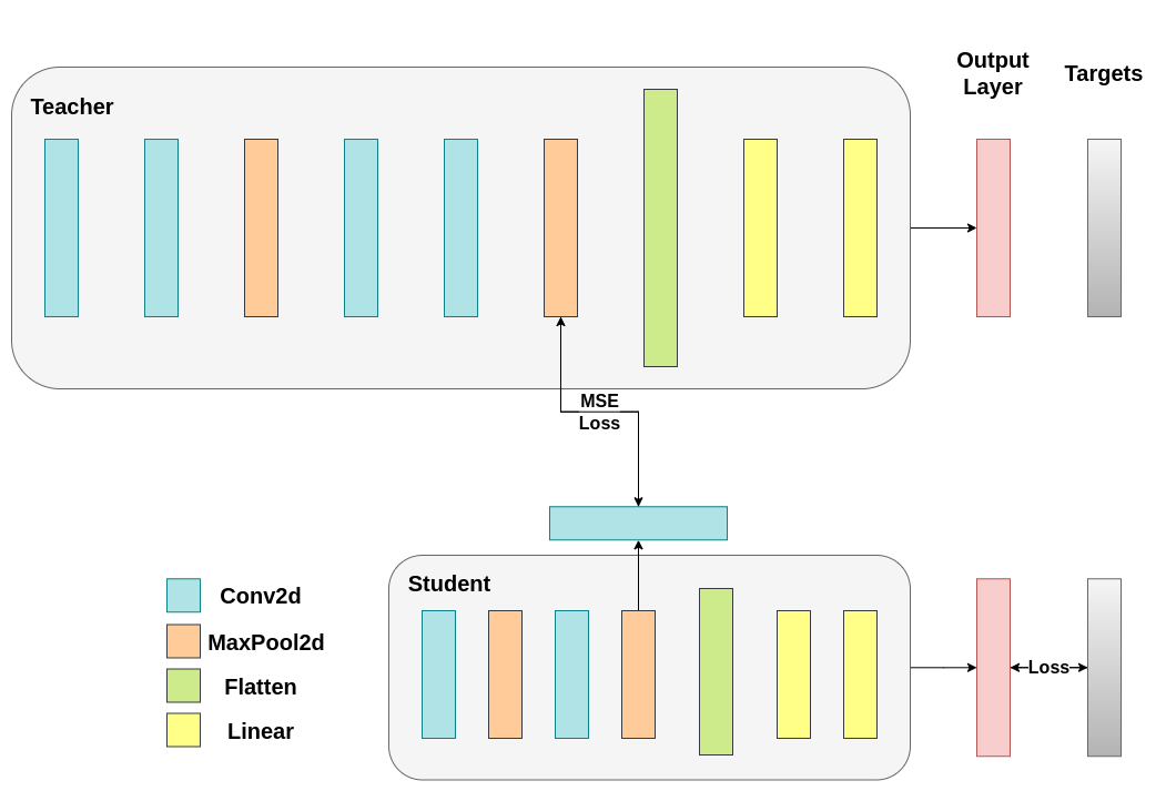
可訓練層匹配中間張量的形狀，並且可以正確定義均方誤差 (MSE)：

class ModifiedDeepNNRegressor(nn.Module):
    def __init__(self, num_classes=10):
        super(ModifiedDeepNNRegressor, self).__init__()
        self.features = nn.Sequential(
            nn.Conv2d(3, 128, kernel_size=3, padding=1),
            nn.ReLU(),
            nn.Conv2d(128, 64, kernel_size=3, padding=1),
            nn.ReLU(),
            nn.MaxPool2d(kernel_size=2, stride=2),
            nn.Conv2d(64, 64, kernel_size=3, padding=1),
            nn.ReLU(),
            nn.Conv2d(64, 32, kernel_size=3, padding=1),
            nn.ReLU(),
            nn.MaxPool2d(kernel_size=2, stride=2),
        )
        self.classifier = nn.Sequential(
            nn.Linear(2048, 512),
            nn.ReLU(),
            nn.Dropout(0.1),
            nn.Linear(512, num_classes)
        )

    def forward(self, x):
        x = self.features(x)
        conv_feature_map = x
        x = torch.flatten(x, 1)
        x = self.classifier(x)
        return x, conv_feature_map

class ModifiedLightNNRegressor(nn.Module):
    def __init__(self, num_classes=10):
        super(ModifiedLightNNRegressor, self).__init__()
        self.features = nn.Sequential(
            nn.Conv2d(3, 16, kernel_size=3, padding=1),
            nn.ReLU(),
            nn.MaxPool2d(kernel_size=2, stride=2),
            nn.Conv2d(16, 16, kernel_size=3, padding=1),
            nn.ReLU(),
            nn.MaxPool2d(kernel_size=2, stride=2),
        )
        # Include an extra regressor (in our case linear)
        self.regressor = nn.Sequential(
            nn.Conv2d(16, 32, kernel_size=3, padding=1)
        )
        self.classifier = nn.Sequential(
            nn.Linear(1024, 256),
            nn.ReLU(),
            nn.Dropout(0.1),
            nn.Linear(256, num_classes)
        )

    def forward(self, x):
        x = self.features(x)
        regressor_output = self.regressor(x)
        x = torch.flatten(x, 1)
        x = self.classifier(x)
        return x, regressor_output

在那之後，我們必須再次更新我們的訓練迴圈。這次，我們提取學生模型的迴歸器輸出，教師模型的中間層特徵圖。然後，我們在這些張量上計算 MSE (它們的形狀完全相同，所以可以正確地定義)，並且根據這個損失來反向傳播梯度，此外還有分類任務的常規交叉熵損失。

def train_mse_loss(teacher, student, train_loader, epochs, learning_rate, feature_map_weight, ce_loss_weight, device):
    ce_loss = nn.CrossEntropyLoss()
    mse_loss = nn.MSELoss()
    optimizer = optim.Adam(student.parameters(), lr=learning_rate)

    teacher.to(device)
    student.to(device)
    teacher.eval()  # Teacher set to evaluation mode
    student.train() # Student to train mode

    for epoch in range(epochs):
        running_loss = 0.0
        for inputs, labels in train_loader:
            inputs, labels = inputs.to(device), labels.to(device)

            optimizer.zero_grad()

            # Again ignore teacher logits
            with torch.no_grad():
                _, teacher_feature_map = teacher(inputs)

            # Forward pass with the student model
            student_logits, regressor_feature_map = student(inputs)

            # Calculate the loss
            hidden_rep_loss = mse_loss(regressor_feature_map, teacher_feature_map)

            # Calculate the true label loss
            label_loss = ce_loss(student_logits, labels)

            # Weighted sum of the two losses
            loss = feature_map_weight * hidden_rep_loss + ce_loss_weight * label_loss

            loss.backward()
            optimizer.step()

            running_loss += loss.item()

        print(f"Epoch {epoch+1}/{epochs}, Loss: {running_loss / len(train_loader)}")

# Notice how our test function remains the same here with the one we used in our previous case. We only care about the actual outputs because we measure accuracy.

# Initialize a ModifiedLightNNRegressor
torch.manual_seed(42)
modified_nn_light_reg = ModifiedLightNNRegressor(num_classes=10).to(device)

# We do not have to train the modified deep network from scratch of course, we just load its weights from the trained instance
modified_nn_deep_reg = ModifiedDeepNNRegressor(num_classes=10).to(device)
modified_nn_deep_reg.load_state_dict(nn_deep.state_dict())

# Train and test once again
train_mse_loss(teacher=modified_nn_deep_reg, student=modified_nn_light_reg, train_loader=train_loader, epochs=10, learning_rate=0.001, feature_map_weight=0.25, ce_loss_weight=0.75, device=device)
test_accuracy_light_ce_and_mse_loss = test_multiple_outputs(modified_nn_light_reg, test_loader, device)

Epoch 1/10, Loss: 1.7066363266971716
Epoch 2/10, Loss: 1.3309815390335629
Epoch 3/10, Loss: 1.188617759196045
Epoch 4/10, Loss: 1.0923469258696221
Epoch 5/10, Loss: 1.0123476643696465
Epoch 6/10, Loss: 0.9512547259135624
Epoch 7/10, Loss: 0.8982603129218606
Epoch 8/10, Loss: 0.8485838961418327
Epoch 9/10, Loss: 0.8041575365054333
Epoch 10/10, Loss: 0.7658210701649756
Test Accuracy: 70.61%

預期最終的方法會比 CosineLoss 更好，因為現在我們允許在教師模型和學生模型之間有一個可訓練的層，這給了學生模型在學習時一些彈性空間，而不是強迫學生複製教師模型的表示。包含額外的網路是基於提示的知識蒸餾背後的想法。

print(f"Teacher accuracy: {test_accuracy_deep:.2f}%")
print(f"Student accuracy without teacher: {test_accuracy_light_ce:.2f}%")
print(f"Student accuracy with CE + KD: {test_accuracy_light_ce_and_kd:.2f}%")
print(f"Student accuracy with CE + CosineLoss: {test_accuracy_light_ce_and_cosine_loss:.2f}%")
print(f"Student accuracy with CE + RegressorMSE: {test_accuracy_light_ce_and_mse_loss:.2f}%")

Teacher accuracy: 75.98%
Student accuracy without teacher: 70.65%
Student accuracy with CE + KD: 70.49%
Student accuracy with CE + CosineLoss: 70.12%
Student accuracy with CE + RegressorMSE: 70.61%

結論

以上任何方法都沒有增加網路的參數數量或推論時間，因此效能的提升來自於在訓練期間計算梯度的少量成本。在 ML 應用程式中，我們主要關心推論時間，因為訓練發生在模型部署之前。如果我們輕量級模型對於部署來說仍然太重，我們可以應用不同的想法，例如訓練後量化。額外的損失可以應用於許多任務，而不僅僅是分類，您可以試驗係數、溫度或神經元數量等數量。您可以隨意調整上面教程中的任何數字，但請記住，如果您更改神經元/過濾器的數量，很可能會發生形狀不匹配。

更多資訊，請參閱：

• Hinton, G., Vinyals, O., Dean, J.: Distilling the knowledge in a neural network. In: Neural Information Processing System Deep Learning Workshop (2015)

• Romero, A., Ballas, N., Kahou, S.E., Chassang, A., Gatta, C., Bengio, Y.: Fitnets: Hints for thin deep nets. In: Proceedings of the International Conference on Learning Representations (2015)