注意
點擊這裡下載完整的範例程式碼
電腦視覺的遷移學習教學
建立時間:2017 年 3 月 24 日 | 最後更新時間:2025 年 1 月 27 日 | 最後驗證時間:2024 年 11 月 05 日
在本教學中,您將學習如何使用遷移學習訓練用於圖像分類的卷積神經網路。您可以在cs231n 筆記中閱讀更多關於遷移學習的資訊
引用這些筆記,
實際上,很少有人從頭開始(使用隨機初始化)訓練整個卷積神經網路,因為擁有足夠大的資料集相對罕見。 相反,通常的做法是在一個非常大的資料集(例如,包含 120 萬張圖片和 1000 個類別的 ImageNet)上預訓練一個 ConvNet,然後將該 ConvNet 用作初始化或固定特徵提取器,以用於感興趣的任務。
以下是這兩個主要的遷移學習情境
微調 ConvNet:我們不使用隨機初始化,而是使用預訓練網路初始化網路,例如在 imagenet 1000 資料集上訓練的網路。 其餘的訓練看起來與往常一樣。
ConvNet 作為固定特徵提取器:在這裡,我們將凍結網路的所有權重,除了最後一個全連接層的權重。 這個最後的全連接層將被一個新的隨機權重層取代,並且僅訓練該層。
# License: BSD
# Author: Sasank Chilamkurthy

import torch
import torch.nn as nn
import torch.optim as optim
from torch.optim import lr_scheduler
import torch.backends.cudnn as cudnn
import numpy as np
import torchvision
from torchvision import datasets, models, transforms
import matplotlib.pyplot as plt
import time
import os
from PIL import Image
from tempfile import TemporaryDirectory

cudnn.benchmark = True
plt.ion()   # interactive mode
<contextlib.ExitStack object at 0x7fb13e4ba860>
載入資料
我們將使用 torchvision 和 torch.utils.data 套件來載入資料。
我們今天要解決的問題是訓練一個模型來分類螞蟻和蜜蜂。 我們分別有大約 120 張用於訓練螞蟻和蜜蜂的圖像。 每個類別有 75 張驗證圖像。 通常,如果從頭開始訓練,這是一個非常小的資料集,無法進行泛化。 由於我們使用的是遷移學習,因此我們應該能夠相當好地泛化。
此資料集是 imagenet 的一個非常小的子集。
注意
從這裡下載資料並將其解壓縮到目前目錄。
# Data augmentation and normalization for training
# Just normalization for validation
data_transforms = {
    'train': transforms.Compose([
        transforms.RandomResizedCrop(224),
        transforms.RandomHorizontalFlip(),
        transforms.ToTensor(),
        transforms.Normalize([0.485, 0.456, 0.406], [0.229, 0.224, 0.225])
    ]),
    'val': transforms.Compose([
        transforms.Resize(256),
        transforms.CenterCrop(224),
        transforms.ToTensor(),
        transforms.Normalize([0.485, 0.456, 0.406], [0.229, 0.224, 0.225])
    ]),
}

data_dir = 'data/hymenoptera_data'
image_datasets = {x: datasets.ImageFolder(os.path.join(data_dir, x),
                                          data_transforms[x])
                  for x in ['train', 'val']}
dataloaders = {x: torch.utils.data.DataLoader(image_datasets[x], batch_size=4,
                                             shuffle=True, num_workers=4)
              for x in ['train', 'val']}
dataset_sizes = {x: len(image_datasets[x]) for x in ['train', 'val']}
class_names = image_datasets['train'].classes

# We want to be able to train our model on an `accelerator <https://pytorch.dev.org.tw/docs/stable/torch.html#accelerators>`__
# such as CUDA, MPS, MTIA, or XPU. If the current accelerator is available, we will use it. Otherwise, we use the CPU.

device = torch.accelerator.current_accelerator().type if torch.accelerator.is_available() else "cpu"
print(f"Using {device} device")
Using cuda device
視覺化一些圖像
讓我們視覺化一些訓練圖像,以便了解資料擴增。
def imshow(inp, title=None):
    """Display image for Tensor."""
    inp = inp.numpy().transpose((1, 2, 0))
    mean = np.array([0.485, 0.456, 0.406])
    std = np.array([0.229, 0.224, 0.225])
    inp = std * inp + mean
    inp = np.clip(inp, 0, 1)
    plt.imshow(inp)
    if title is not None:
        plt.title(title)
    plt.pause(0.001)  # pause a bit so that plots are updated


# Get a batch of training data
inputs, classes = next(iter(dataloaders['train']))

# Make a grid from batch
out = torchvision.utils.make_grid(inputs)

imshow(out, title=[class_names[x] for x in classes])
![['ants', 'ants', 'ants', 'ants']](../_images/sphx_glr_transfer_learning_tutorial_001.png)
訓練模型
現在,讓我們編寫一個通用函數來訓練模型。 在這裡,我們將說明
排程學習速率
儲存最佳模型
在以下程式碼中,參數 scheduler 是來自 torch.optim.lr_scheduler 的 LR 排程器物件。
def train_model(model, criterion, optimizer, scheduler, num_epochs=25):
    since = time.time()

    # Create a temporary directory to save training checkpoints
    with TemporaryDirectory() as tempdir:
        best_model_params_path = os.path.join(tempdir, 'best_model_params.pt')

        torch.save(model.state_dict(), best_model_params_path)
        best_acc = 0.0

        for epoch in range(num_epochs):
            print(f'Epoch {epoch}/{num_epochs - 1}')
            print('-' * 10)

            # Each epoch has a training and validation phase
            for phase in ['train', 'val']:
                if phase == 'train':
                    model.train()  # Set model to training mode
                else:
                    model.eval()   # Set model to evaluate mode

                running_loss = 0.0
                running_corrects = 0

                # Iterate over data.
                for inputs, labels in dataloaders[phase]:
                    inputs = inputs.to(device)
                    labels = labels.to(device)

                    # zero the parameter gradients
                    optimizer.zero_grad()

                    # forward
                    # track history if only in train
                    with torch.set_grad_enabled(phase == 'train'):
                        outputs = model(inputs)
                        _, preds = torch.max(outputs, 1)
                        loss = criterion(outputs, labels)

                        # backward + optimize only if in training phase
                        if phase == 'train':
                            loss.backward()
                            optimizer.step()

                    # statistics
                    running_loss += loss.item() * inputs.size(0)
                    running_corrects += torch.sum(preds == labels.data)
                if phase == 'train':
                    scheduler.step()

                epoch_loss = running_loss / dataset_sizes[phase]
                epoch_acc = running_corrects.double() / dataset_sizes[phase]

                print(f'{phase} Loss: {epoch_loss:.4f} Acc: {epoch_acc:.4f}')

                # deep copy the model
                if phase == 'val' and epoch_acc > best_acc:
                    best_acc = epoch_acc
                    torch.save(model.state_dict(), best_model_params_path)

            print()

        time_elapsed = time.time() - since
        print(f'Training complete in {time_elapsed // 60:.0f}m {time_elapsed % 60:.0f}s')
        print(f'Best val Acc: {best_acc:4f}')

        # load best model weights
        model.load_state_dict(torch.load(best_model_params_path, weights_only=True))
    return model
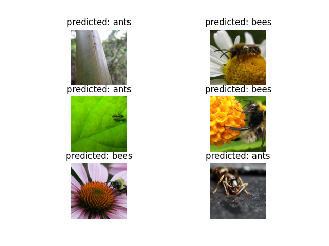
視覺化模型預測
用於顯示一些圖像的預測的通用函數
def visualize_model(model, num_images=6):
    was_training = model.training
    model.eval()
    images_so_far = 0
    fig = plt.figure()

    with torch.no_grad():
        for i, (inputs, labels) in enumerate(dataloaders['val']):
            inputs = inputs.to(device)
            labels = labels.to(device)

            outputs = model(inputs)
            _, preds = torch.max(outputs, 1)

            for j in range(inputs.size()[0]):
                images_so_far += 1
                ax = plt.subplot(num_images//2, 2, images_so_far)
                ax.axis('off')
                ax.set_title(f'predicted: {class_names[preds[j]]}')
                imshow(inputs.cpu().data[j])

                if images_so_far == num_images:
                    model.train(mode=was_training)
                    return
        model.train(mode=was_training)
微調 ConvNet
載入預訓練模型並重設最後一個全連接層。
model_ft = models.resnet18(weights='IMAGENET1K_V1')
num_ftrs = model_ft.fc.in_features
# Here the size of each output sample is set to 2.
# Alternatively, it can be generalized to ``nn.Linear(num_ftrs, len(class_names))``.
model_ft.fc = nn.Linear(num_ftrs, 2)

model_ft = model_ft.to(device)

criterion = nn.CrossEntropyLoss()

# Observe that all parameters are being optimized
optimizer_ft = optim.SGD(model_ft.parameters(), lr=0.001, momentum=0.9)

# Decay LR by a factor of 0.1 every 7 epochs
exp_lr_scheduler = lr_scheduler.StepLR(optimizer_ft, step_size=7, gamma=0.1)
Downloading: "https://download.pytorch.org/models/resnet18-f37072fd.pth" to /var/lib/ci-user/.cache/torch/hub/checkpoints/resnet18-f37072fd.pth

  0%|          | 0.00/44.7M [00:00<?, ?B/s]
 46%|####6     | 20.6M/44.7M [00:00<00:00, 216MB/s]
 93%|#########3| 41.8M/44.7M [00:00<00:00, 219MB/s]
100%|##########| 44.7M/44.7M [00:00<00:00, 219MB/s]
訓練和評估
在 CPU 上大約需要 15-25 分鐘。 但是,在 GPU 上,所需時間不到一分鐘。
model_ft = train_model(model_ft, criterion, optimizer_ft, exp_lr_scheduler,
                       num_epochs=25)
Epoch 0/24
----------
train Loss: 0.4763 Acc: 0.7623
val Loss: 0.2740 Acc: 0.8889

Epoch 1/24
----------
train Loss: 0.5324 Acc: 0.7992
val Loss: 0.6551 Acc: 0.7386

Epoch 2/24
----------
train Loss: 0.4263 Acc: 0.8238
val Loss: 0.2401 Acc: 0.9150

Epoch 3/24
----------
train Loss: 0.5954 Acc: 0.7582
val Loss: 0.2763 Acc: 0.9020

Epoch 4/24
----------
train Loss: 0.3802 Acc: 0.8361
val Loss: 0.2835 Acc: 0.9085

Epoch 5/24
----------
train Loss: 0.4481 Acc: 0.8033
val Loss: 0.2775 Acc: 0.8954

Epoch 6/24
----------
train Loss: 0.3503 Acc: 0.8115
val Loss: 0.2096 Acc: 0.9216

Epoch 7/24
----------
train Loss: 0.3870 Acc: 0.8689
val Loss: 0.1859 Acc: 0.9412

Epoch 8/24
----------
train Loss: 0.2612 Acc: 0.9098
val Loss: 0.1868 Acc: 0.9281

Epoch 9/24
----------
train Loss: 0.2483 Acc: 0.8893
val Loss: 0.2420 Acc: 0.9150

Epoch 10/24
----------
train Loss: 0.3824 Acc: 0.8484
val Loss: 0.1724 Acc: 0.9477

Epoch 11/24
----------
train Loss: 0.3602 Acc: 0.8279
val Loss: 0.2520 Acc: 0.9020

Epoch 12/24
----------
train Loss: 0.2301 Acc: 0.8934
val Loss: 0.2084 Acc: 0.9216

Epoch 13/24
----------
train Loss: 0.3166 Acc: 0.8770
val Loss: 0.1766 Acc: 0.9412

Epoch 14/24
----------
train Loss: 0.2658 Acc: 0.8893
val Loss: 0.2410 Acc: 0.8824

Epoch 15/24
----------
train Loss: 0.3039 Acc: 0.8607
val Loss: 0.2693 Acc: 0.8693

Epoch 16/24
----------
train Loss: 0.2393 Acc: 0.9016
val Loss: 0.1950 Acc: 0.9216

Epoch 17/24
----------
train Loss: 0.2621 Acc: 0.8975
val Loss: 0.1714 Acc: 0.9412

Epoch 18/24
----------
train Loss: 0.3069 Acc: 0.8893
val Loss: 0.1892 Acc: 0.9216

Epoch 19/24
----------
train Loss: 0.2038 Acc: 0.9221
val Loss: 0.1868 Acc: 0.9150

Epoch 20/24
----------
train Loss: 0.2525 Acc: 0.8975
val Loss: 0.1897 Acc: 0.9281

Epoch 21/24
----------
train Loss: 0.2515 Acc: 0.8852
val Loss: 0.2172 Acc: 0.9020

Epoch 22/24
----------
train Loss: 0.3098 Acc: 0.8730
val Loss: 0.1718 Acc: 0.9412

Epoch 23/24
----------
train Loss: 0.2756 Acc: 0.8730
val Loss: 0.2057 Acc: 0.9216

Epoch 24/24
----------
train Loss: 0.2886 Acc: 0.8852
val Loss: 0.1722 Acc: 0.9542

Training complete in 1m 4s
Best val Acc: 0.954248
visualize_model(model_ft)
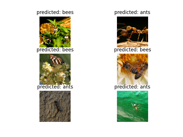
ConvNet 作為固定特徵提取器
在這裡,我們需要凍結除了最後一層之外的所有網路。 我們需要設定 requires_grad = False 以凍結參數,以便在 backward() 中不計算梯度。
您可以在此處的文件中閱讀更多相關資訊。
model_conv = torchvision.models.resnet18(weights='IMAGENET1K_V1')
for param in model_conv.parameters():
    param.requires_grad = False

# Parameters of newly constructed modules have requires_grad=True by default
num_ftrs = model_conv.fc.in_features
model_conv.fc = nn.Linear(num_ftrs, 2)

model_conv = model_conv.to(device)

criterion = nn.CrossEntropyLoss()

# Observe that only parameters of final layer are being optimized as
# opposed to before.
optimizer_conv = optim.SGD(model_conv.fc.parameters(), lr=0.001, momentum=0.9)

# Decay LR by a factor of 0.1 every 7 epochs
exp_lr_scheduler = lr_scheduler.StepLR(optimizer_conv, step_size=7, gamma=0.1)
訓練和評估
與先前的場景相比,在 CPU 上,這將花費大約一半的時間。 這是預期的,因為不需要為大多數網路計算梯度。 但是,確實需要計算前向傳播。
model_conv = train_model(model_conv, criterion, optimizer_conv,
                         exp_lr_scheduler, num_epochs=25)
Epoch 0/24
----------
train Loss: 0.6996 Acc: 0.6516
val Loss: 0.2014 Acc: 0.9346

Epoch 1/24
----------
train Loss: 0.4233 Acc: 0.8033
val Loss: 0.2656 Acc: 0.8758

Epoch 2/24
----------
train Loss: 0.4603 Acc: 0.7869
val Loss: 0.1847 Acc: 0.9477

Epoch 3/24
----------
train Loss: 0.3096 Acc: 0.8566
val Loss: 0.1747 Acc: 0.9477

Epoch 4/24
----------
train Loss: 0.4427 Acc: 0.8156
val Loss: 0.1630 Acc: 0.9477

Epoch 5/24
----------
train Loss: 0.5505 Acc: 0.7828
val Loss: 0.1643 Acc: 0.9477

Epoch 6/24
----------
train Loss: 0.3004 Acc: 0.8607
val Loss: 0.1744 Acc: 0.9542

Epoch 7/24
----------
train Loss: 0.4083 Acc: 0.8361
val Loss: 0.1892 Acc: 0.9412

Epoch 8/24
----------
train Loss: 0.4483 Acc: 0.7910
val Loss: 0.1984 Acc: 0.9477

Epoch 9/24
----------
train Loss: 0.3335 Acc: 0.8279
val Loss: 0.1942 Acc: 0.9412

Epoch 10/24
----------
train Loss: 0.2413 Acc: 0.8934
val Loss: 0.2001 Acc: 0.9477

Epoch 11/24
----------
train Loss: 0.3107 Acc: 0.8689
val Loss: 0.1801 Acc: 0.9412

Epoch 12/24
----------
train Loss: 0.3032 Acc: 0.8689
val Loss: 0.1669 Acc: 0.9477

Epoch 13/24
----------
train Loss: 0.3587 Acc: 0.8525
val Loss: 0.1900 Acc: 0.9477

Epoch 14/24
----------
train Loss: 0.2771 Acc: 0.8893
val Loss: 0.2317 Acc: 0.9216

Epoch 15/24
----------
train Loss: 0.3064 Acc: 0.8852
val Loss: 0.1909 Acc: 0.9477

Epoch 16/24
----------
train Loss: 0.4243 Acc: 0.8238
val Loss: 0.2227 Acc: 0.9346

Epoch 17/24
----------
train Loss: 0.3297 Acc: 0.8238
val Loss: 0.1916 Acc: 0.9412

Epoch 18/24
----------
train Loss: 0.4235 Acc: 0.8238
val Loss: 0.1766 Acc: 0.9477

Epoch 19/24
----------
train Loss: 0.2500 Acc: 0.8934
val Loss: 0.2003 Acc: 0.9477

Epoch 20/24
----------
train Loss: 0.2413 Acc: 0.8934
val Loss: 0.1821 Acc: 0.9477

Epoch 21/24
----------
train Loss: 0.3762 Acc: 0.8115
val Loss: 0.1842 Acc: 0.9412

Epoch 22/24
----------
train Loss: 0.3485 Acc: 0.8566
val Loss: 0.2166 Acc: 0.9281

Epoch 23/24
----------
train Loss: 0.3625 Acc: 0.8361
val Loss: 0.1747 Acc: 0.9412

Epoch 24/24
----------
train Loss: 0.3840 Acc: 0.8320
val Loss: 0.1768 Acc: 0.9412

Training complete in 0m 32s
Best val Acc: 0.954248
visualize_model(model_conv)

plt.ioff()
plt.show()
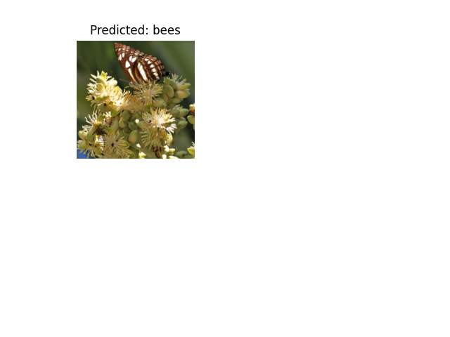
自定義圖像的推論
使用訓練好的模型對自定義圖像進行預測,並視覺化預測的類別標籤以及圖像。
def visualize_model_predictions(model,img_path):
    was_training = model.training
    model.eval()

    img = Image.open(img_path)
    img = data_transforms['val'](img)
    img = img.unsqueeze(0)
    img = img.to(device)

    with torch.no_grad():
        outputs = model(img)
        _, preds = torch.max(outputs, 1)

        ax = plt.subplot(2,2,1)
        ax.axis('off')
        ax.set_title(f'Predicted: {class_names[preds[0]]}')
        imshow(img.cpu().data[0])

        model.train(mode=was_training)
visualize_model_predictions(
    model_conv,
    img_path='data/hymenoptera_data/val/bees/72100438_73de9f17af.jpg'
)

plt.ioff()
plt.show()