


注意
點擊這裡下載完整的範例程式碼
使用 Hybrid Demucs 進行音樂源分離
作者:Sean Kim
本教學展示如何使用 Hybrid Demucs 模型來執行音樂分離
1. 概述
執行音樂分離包含以下步驟
建置 Hybrid Demucs 管線。
將波形格式化為預期大小的區塊,並迴圈處理區塊(帶有重疊),然後饋入管線。
收集輸出區塊並根據它們的重疊方式組合。
Hybrid Demucs [Défossez, 2021] 模型是 Demucs 模型的開發版本,這是一個基於波形的模型,可將音樂分離為其各自的來源,例如人聲、貝斯和鼓。 Hybrid Demucs 有效地使用頻譜圖來通過頻域學習,並且還轉向時間卷積。
2. 準備
首先,我們安裝必要的相依性。第一個要求是 torchaudio 和 torch
import torch
import torchaudio
print(torch.__version__)
print(torchaudio.__version__)
import matplotlib.pyplot as plt
2.6.0
2.6.0
除了 torchaudio 之外,還需要 mir_eval 才能執行訊號失真比 (SDR) 計算。 要安裝 mir_eval,請使用 pip3 install mir_eval。
from IPython.display import Audio
from mir_eval import separation
from torchaudio.pipelines import HDEMUCS_HIGH_MUSDB_PLUS
from torchaudio.utils import download_asset
3. 構建管線
預先訓練的模型權重和相關的管線組件被捆綁為 torchaudio.pipelines.HDEMUCS_HIGH_MUSDB_PLUS()。 這是一個在 MUSDB18-HQ 和額外的內部訓練數據上訓練的 torchaudio.models.HDemucs 模型。 這個特定的模型適用於較高的取樣率,約為 44.1 kHZ,並且在模型實現中具有 4096 的 nfft 值和 6 的深度。
bundle = HDEMUCS_HIGH_MUSDB_PLUS
model = bundle.get_model()
device = torch.device("cuda:0" if torch.cuda.is_available() else "cpu")
model.to(device)
sample_rate = bundle.sample_rate
print(f"Sample rate: {sample_rate}")
0%| | 0.00/319M [00:00<?, ?B/s]
14%|#3 | 44.5M/319M [00:00<00:00, 467MB/s]
28%|##7 | 89.0M/319M [00:00<00:00, 463MB/s]
42%|####1 | 133M/319M [00:00<00:00, 455MB/s]
55%|#####5 | 177M/319M [00:00<00:00, 445MB/s]
69%|######9 | 221M/319M [00:00<00:00, 451MB/s]
83%|########2 | 264M/319M [00:00<00:00, 431MB/s]
97%|#########7| 310M/319M [00:00<00:00, 447MB/s]
100%|##########| 319M/319M [00:00<00:00, 445MB/s]
/pytorch/audio/src/torchaudio/pipelines/_source_separation_pipeline.py:56: FutureWarning: You are using `torch.load` with `weights_only=False` (the current default value), which uses the default pickle module implicitly. It is possible to construct malicious pickle data which will execute arbitrary code during unpickling (See https://github.com/pytorch/pytorch/blob/main/SECURITY.md#untrusted-models for more details). In a future release, the default value for `weights_only` will be flipped to `True`. This limits the functions that could be executed during unpickling. Arbitrary objects will no longer be allowed to be loaded via this mode unless they are explicitly allowlisted by the user via `torch.serialization.add_safe_globals`. We recommend you start setting `weights_only=True` for any use case where you don't have full control of the loaded file. Please open an issue on GitHub for any issues related to this experimental feature.
state_dict = torch.load(path)
Sample rate: 44100
4. 配置應用程式函數
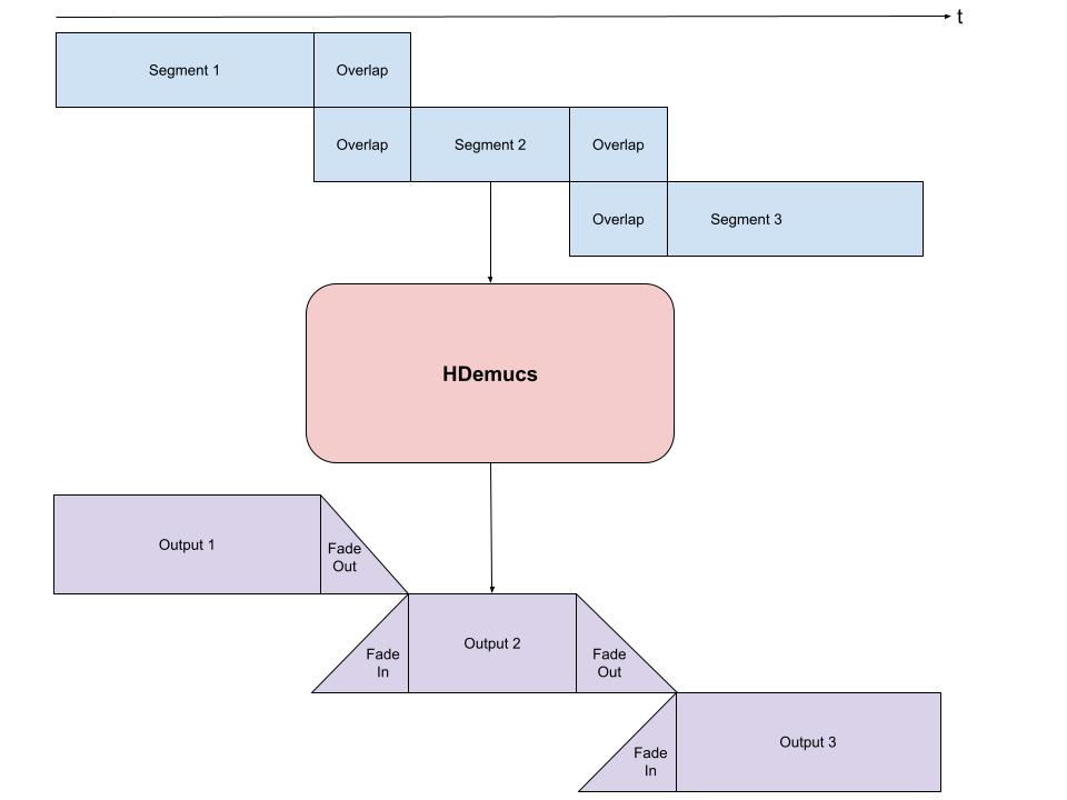
由於 HDemucs 是一個大型且消耗記憶體的模型,因此很難有足夠的記憶體一次將模型應用於整首歌曲。 為了克服這個限制,將歌曲分塊成更小的片段,逐一執行模型,然後重新組合在一起,以獲得完整歌曲的分離音源。
在這樣做時,重要的是確保每個塊之間有一些重疊,以適應邊緣的偽像。 由於模型的性質,有時邊緣包含不準確或不需要的聲音。
我們在下面提供了一個分塊和排列的示例實現。 這個實現在每一側都採用 1 秒的重疊,然後在每一側進行線性淡入和淡出。 使用淡化的重疊部分,我將這些片段加在一起,以確保整個過程保持恆定的音量。 這通過減少模型輸出的邊緣使用量來適應偽像。
from torchaudio.transforms import Fade
def separate_sources(
model,
mix,
segment=10.0,
overlap=0.1,
device=None,
):
"""
Apply model to a given mixture. Use fade, and add segments together in order to add model segment by segment.
Args:
segment (int): segment length in seconds
device (torch.device, str, or None): if provided, device on which to
execute the computation, otherwise `mix.device` is assumed.
When `device` is different from `mix.device`, only local computations will
be on `device`, while the entire tracks will be stored on `mix.device`.
"""
if device is None:
device = mix.device
else:
device = torch.device(device)
batch, channels, length = mix.shape
chunk_len = int(sample_rate * segment * (1 + overlap))
start = 0
end = chunk_len
overlap_frames = overlap * sample_rate
fade = Fade(fade_in_len=0, fade_out_len=int(overlap_frames), fade_shape="linear")
final = torch.zeros(batch, len(model.sources), channels, length, device=device)
while start < length - overlap_frames:
chunk = mix[:, :, start:end]
with torch.no_grad():
out = model.forward(chunk)
out = fade(out)
final[:, :, :, start:end] += out
if start == 0:
fade.fade_in_len = int(overlap_frames)
start += int(chunk_len - overlap_frames)
else:
start += chunk_len
end += chunk_len
if end >= length:
fade.fade_out_len = 0
return final
def plot_spectrogram(stft, title="Spectrogram"):
magnitude = stft.abs()
spectrogram = 20 * torch.log10(magnitude + 1e-8).numpy()
_, axis = plt.subplots(1, 1)
axis.imshow(spectrogram, cmap="viridis", vmin=-60, vmax=0, origin="lower", aspect="auto")
axis.set_title(title)
plt.tight_layout()
5. 執行模型
最後,我們執行模型並將單獨的音源檔案儲存在目錄中
作為測試歌曲,我們將使用 MedleyDB 中 NightOwl 的 A Classic Education(Creative Commons BY-NC-SA 4.0)。 這也位於 MUSDB18-HQ 數據集中 train 音源中。
為了用不同的歌曲進行測試,可以更改下面的變數名稱和網址,以及參數,以不同的方式測試歌曲分離器。
# We download the audio file from our storage. Feel free to download another file and use audio from a specific path
SAMPLE_SONG = download_asset("tutorial-assets/hdemucs_mix.wav")
waveform, sample_rate = torchaudio.load(SAMPLE_SONG) # replace SAMPLE_SONG with desired path for different song
waveform = waveform.to(device)
mixture = waveform
# parameters
segment: int = 10
overlap = 0.1
print("Separating track")
ref = waveform.mean(0)
waveform = (waveform - ref.mean()) / ref.std() # normalization
sources = separate_sources(
model,
waveform[None],
device=device,
segment=segment,
overlap=overlap,
)[0]
sources = sources * ref.std() + ref.mean()
sources_list = model.sources
sources = list(sources)
audios = dict(zip(sources_list, sources))
0%| | 0.00/28.8M [00:00<?, ?B/s]
57%|#####7 | 16.5M/28.8M [00:00<00:00, 80.7MB/s]
100%|##########| 28.8M/28.8M [00:00<00:00, 104MB/s]
Separating track
5.1 分離音軌
已加載的預訓練權重的默認集有 4 個音源,它被分成:鼓、貝斯、其他和人聲,依此順序。 它們已儲存在 dict “audios” 中,因此可以在那裡訪問。 對於四個音源,每個音源都有一個單獨的儲存格,它將創建音訊、頻譜圖,並計算 SDR 分數。 SDR 是訊號失真比,本質上是音軌“品質”的表示。
N_FFT = 4096
N_HOP = 4
stft = torchaudio.transforms.Spectrogram(
n_fft=N_FFT,
hop_length=N_HOP,
power=None,
)
5.2 音訊分段和處理
以下是處理步驟和分段 5 秒的音軌,以便輸入到頻譜圖並計算各自的 SDR 分數。
def output_results(original_source: torch.Tensor, predicted_source: torch.Tensor, source: str):
print(
"SDR score is:",
separation.bss_eval_sources(original_source.detach().numpy(), predicted_source.detach().numpy())[0].mean(),
)
plot_spectrogram(stft(predicted_source)[0], f"Spectrogram - {source}")
return Audio(predicted_source, rate=sample_rate)
segment_start = 150
segment_end = 155
frame_start = segment_start * sample_rate
frame_end = segment_end * sample_rate
drums_original = download_asset("tutorial-assets/hdemucs_drums_segment.wav")
bass_original = download_asset("tutorial-assets/hdemucs_bass_segment.wav")
vocals_original = download_asset("tutorial-assets/hdemucs_vocals_segment.wav")
other_original = download_asset("tutorial-assets/hdemucs_other_segment.wav")
drums_spec = audios["drums"][:, frame_start:frame_end].cpu()
drums, sample_rate = torchaudio.load(drums_original)
bass_spec = audios["bass"][:, frame_start:frame_end].cpu()
bass, sample_rate = torchaudio.load(bass_original)
vocals_spec = audios["vocals"][:, frame_start:frame_end].cpu()
vocals, sample_rate = torchaudio.load(vocals_original)
other_spec = audios["other"][:, frame_start:frame_end].cpu()
other, sample_rate = torchaudio.load(other_original)
mix_spec = mixture[:, frame_start:frame_end].cpu()
0%| | 0.00/1.68M [00:00<?, ?B/s]
100%|##########| 1.68M/1.68M [00:00<00:00, 67.9MB/s]
0%| | 0.00/1.68M [00:00<?, ?B/s]
100%|##########| 1.68M/1.68M [00:00<00:00, 102MB/s]
0%| | 0.00/1.68M [00:00<?, ?B/s]
100%|##########| 1.68M/1.68M [00:00<00:00, 171MB/s]
0%| | 0.00/1.68M [00:00<?, ?B/s]
100%|##########| 1.68M/1.68M [00:00<00:00, 120MB/s]
5.3 頻譜圖和音訊
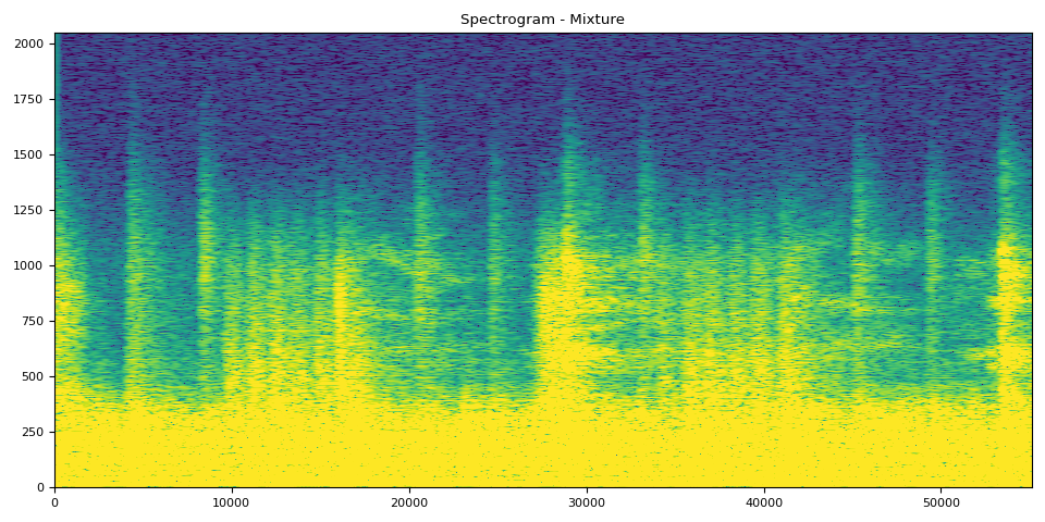
在接下來的 5 個儲存格中,您可以看到帶有各自音訊的頻譜圖。 可以使用頻譜圖清楚地視覺化音訊。
混合剪輯來自原始音軌,其餘音軌是模型輸出
# Mixture Clip
plot_spectrogram(stft(mix_spec)[0], "Spectrogram - Mixture")
Audio(mix_spec, rate=sample_rate)
鼓 SDR、頻譜圖和音訊
# Drums Clip
output_results(drums, drums_spec, "drums")
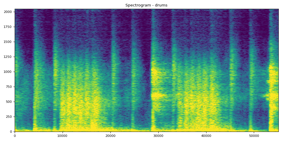
SDR score is: 4.964477475897244
貝斯 SDR、頻譜圖和音訊
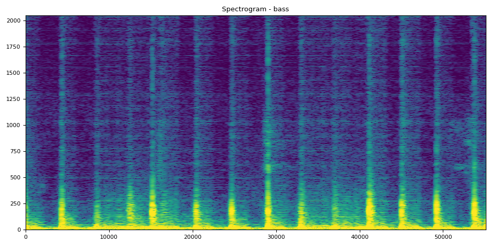
SDR score is: 18.90589959575034
人聲 SDR、頻譜圖和音訊
# Vocals Audio
output_results(vocals, vocals_spec, "vocals")
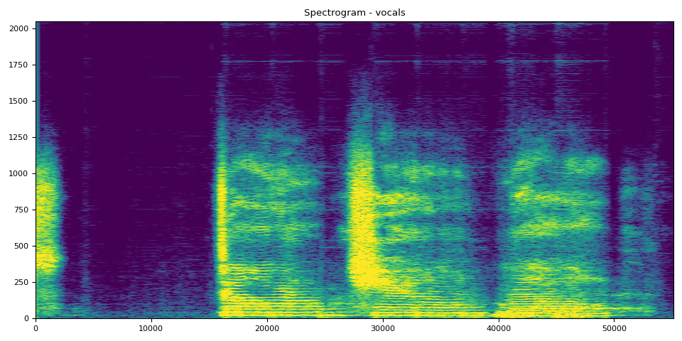
SDR score is: 8.792372276328596
其他 SDR、頻譜圖和音訊
# Other Clip
output_results(other, other_spec, "other")
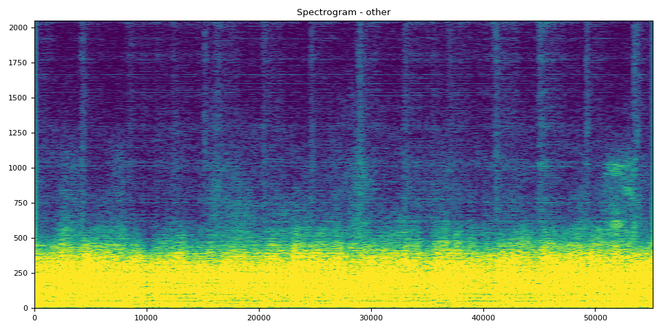
SDR score is: 8.866964245665635
# Optionally, the full audios can be heard in from running the next 5
# cells. They will take a bit longer to load, so to run simply uncomment
# out the ``Audio`` cells for the respective track to produce the audio
# for the full song.
#
# Full Audio
# Audio(mixture, rate=sample_rate)
# Drums Audio
# Audio(audios["drums"], rate=sample_rate)
# Bass Audio
# Audio(audios["bass"], rate=sample_rate)
# Vocals Audio
# Audio(audios["vocals"], rate=sample_rate)
# Other Audio
# Audio(audios["other"], rate=sample_rate)
腳本的總執行時間:(0 分鐘 25.315 秒)
