注意

點擊此處以下載完整的範例程式碼

使用 Wav2Vec2 進行語音辨識¶

作者: Moto Hira

本教學展示如何使用來自 wav2vec 2.0 的預訓練模型執行語音辨識 [論文]。

概述¶

語音辨識的流程如下。

從音訊波形中提取聲學特徵
逐幀估計聲學特徵的類別
從類別機率序列產生假設

Torchaudio 提供對預訓練權重和相關資訊 (例如預期取樣率和類別標籤) 的輕鬆存取。它們捆綁在一起，可在 torchaudio.pipelines 模組下取得。

準備¶

import torch
import torchaudio

print(torch.__version__)
print(torchaudio.__version__)

torch.random.manual_seed(0)
device = torch.device("cuda" if torch.cuda.is_available() else "cpu")

print(device)

2.6.0
2.6.0
cuda

import IPython
import matplotlib.pyplot as plt
from torchaudio.utils import download_asset

SPEECH_FILE = download_asset("tutorial-assets/Lab41-SRI-VOiCES-src-sp0307-ch127535-sg0042.wav")

  0%|          | 0.00/106k [00:00<?, ?B/s]
100%|##########| 106k/106k [00:00<00:00, 62.6MB/s]

建立 Pipeline¶

首先，我們將建立一個執行特徵提取和分類的 Wav2Vec2 模型。

torchaudio 中有兩種可用的 Wav2Vec2 預訓練權重。一種是針對 ASR 任務進行微調的，另一種則沒有。

Wav2Vec2 (和 HuBERT) 模型以自我監督的方式訓練。它們首先僅使用音訊進行表示學習來訓練，然後使用額外的標籤針對特定任務進行微調。

未經微調的預訓練權重也可以針對其他下游任務進行微調，但本教學課程不涵蓋此內容。

我們將在此使用 torchaudio.pipelines.WAV2VEC2_ASR_BASE_960H。

在 torchaudio.pipelines 中有多個預訓練模型可供使用。請查看文件以了解它們的訓練細節。

bundle 物件提供了實例化模型和其他資訊的介面。取樣率和類別標籤如下所示。

bundle = torchaudio.pipelines.WAV2VEC2_ASR_BASE_960H

print("Sample Rate:", bundle.sample_rate)

print("Labels:", bundle.get_labels())

Sample Rate: 16000
Labels: ('-', '|', 'E', 'T', 'A', 'O', 'N', 'I', 'H', 'S', 'R', 'D', 'L', 'U', 'M', 'W', 'C', 'F', 'G', 'Y', 'P', 'B', 'V', 'K', "'", 'X', 'J', 'Q', 'Z')

模型可以如下建構。此過程會自動獲取預訓練權重並將其加載到模型中。

model = bundle.get_model().to(device)

print(model.__class__)

Downloading: "https://download.pytorch.org/torchaudio/models/wav2vec2_fairseq_base_ls960_asr_ls960.pth" to /root/.cache/torch/hub/checkpoints/wav2vec2_fairseq_base_ls960_asr_ls960.pth

  0%|          | 0.00/360M [00:00<?, ?B/s]
 16%|#5        | 56.8M/360M [00:00<00:00, 594MB/s]
 32%|###1      | 114M/360M [00:00<00:00, 595MB/s]
 47%|####7     | 170M/360M [00:00<00:00, 595MB/s]
 63%|######3   | 227M/360M [00:00<00:00, 585MB/s]
 79%|#######8  | 284M/360M [00:00<00:00, 589MB/s]
 95%|#########4| 341M/360M [00:00<00:00, 591MB/s]
100%|##########| 360M/360M [00:00<00:00, 590MB/s]
<class 'torchaudio.models.wav2vec2.model.Wav2Vec2Model'>

載入資料¶

我們將使用來自 VOiCES dataset 的語音資料，該資料集根據 Creative Commons BY 4.0 授權。

IPython.display.Audio(SPEECH_FILE)

為了載入資料，我們使用 torchaudio.load()。

如果取樣率與 pipeline 預期的不同，那麼我們可以使用 torchaudio.functional.resample() 進行重新取樣。

注意

torchaudio.functional.resample() 也適用於 CUDA tensors。
當對同一組取樣率執行多次重新取樣時，使用 torchaudio.transforms.Resample 可能會提高效能。

waveform, sample_rate = torchaudio.load(SPEECH_FILE)
waveform = waveform.to(device)

if sample_rate != bundle.sample_rate:
    waveform = torchaudio.functional.resample(waveform, sample_rate, bundle.sample_rate)

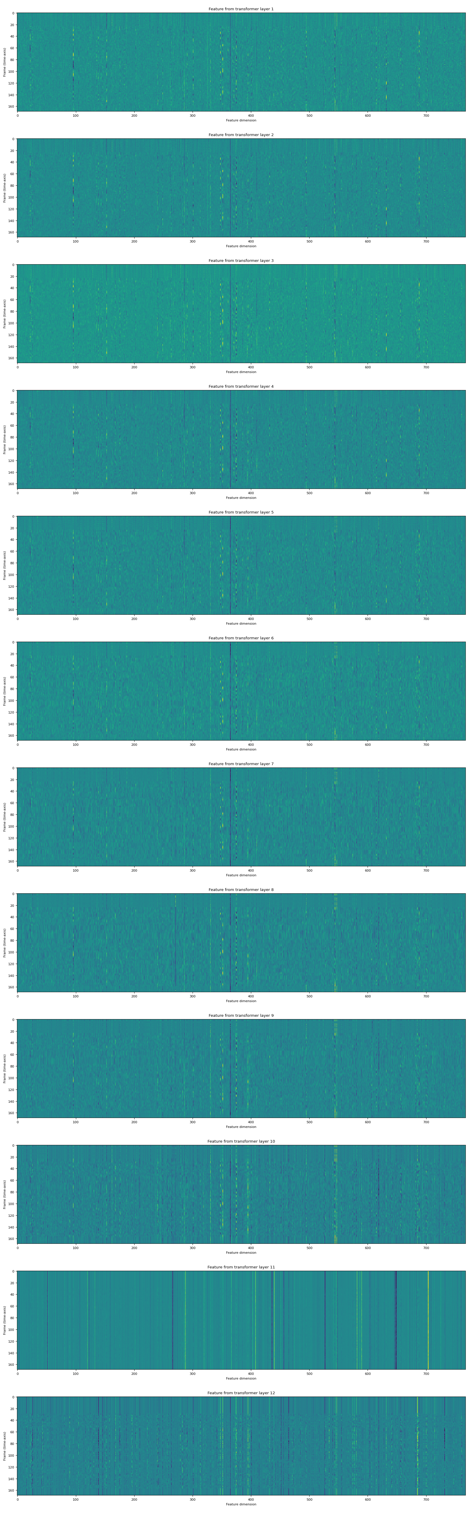
提取聲學特徵¶

下一步是從音訊中提取聲學特徵。

注意

針對 ASR 任務進行微調的 Wav2Vec2 模型可以一步執行特徵提取和分類，但為了本教學的目的，我們也展示如何在此處執行特徵提取。

with torch.inference_mode():
    features, _ = model.extract_features(waveform)

返回的特徵是 tensors 的列表。每個 tensor 都是 transformer 層的輸出。

fig, ax = plt.subplots(len(features), 1, figsize=(16, 4.3 * len(features)))
for i, feats in enumerate(features):
    ax[i].imshow(feats[0].cpu(), interpolation="nearest")
    ax[i].set_title(f"Feature from transformer layer {i+1}")
    ax[i].set_xlabel("Feature dimension")
    ax[i].set_ylabel("Frame (time-axis)")
fig.tight_layout()

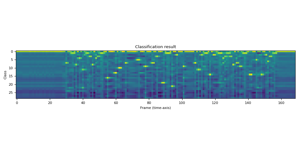
Feature from transformer layer 1, Feature from transformer layer 2, Feature from transformer layer 3, Feature from transformer layer 4, Feature from transformer layer 5, Feature from transformer layer 6, Feature from transformer layer 7, Feature from transformer layer 8, Feature from transformer layer 9, Feature from transformer layer 10, Feature from transformer layer 11, Feature from transformer layer 12

特徵分類¶

提取聲學特徵後，下一步是將它們分類為一組類別。

Wav2Vec2 模型提供了一種方法來一步執行特徵提取和分類。

with torch.inference_mode():
    emission, _ = model(waveform)

輸出採用 logits 的形式。它不是機率的形式。

讓我們將其視覺化。

plt.imshow(emission[0].cpu().T, interpolation="nearest")
plt.title("Classification result")
plt.xlabel("Frame (time-axis)")
plt.ylabel("Class")
plt.tight_layout()
print("Class labels:", bundle.get_labels())

Class labels: ('-', '|', 'E', 'T', 'A', 'O', 'N', 'I', 'H', 'S', 'R', 'D', 'L', 'U', 'M', 'W', 'C', 'F', 'G', 'Y', 'P', 'B', 'V', 'K', "'", 'X', 'J', 'Q', 'Z')

我們可以看見時間軸上對某些標籤有強烈的指示。

生成文本¶

從標籤機率序列，現在我們想要生成文本。生成假設的過程通常稱為「解碼」。

解碼比簡單分類更複雜，因為某個時間步長的解碼可能會受到周圍觀察的影響。

例如，以 night 和 knight 這樣的詞為例。即使它們的先驗機率分佈不同（在典型的對話中，night 的出現頻率遠高於 knight），為了準確地生成包含 knight 的文本，例如 a knight with a sword，解碼過程必須推遲最終決定，直到看到足夠的上下文。

已經提出了許多解碼技術，並且它們需要外部資源，例如單詞詞典和語言模型。

在本教程中，為了簡單起見，我們將執行貪婪解碼，該解碼不依賴於此類外部組件，並且僅簡單地選擇每個時間步長的最佳假設。因此，不使用上下文資訊，並且只能生成一個文本。

我們首先定義貪婪解碼演算法。

class GreedyCTCDecoder(torch.nn.Module):
    def __init__(self, labels, blank=0):
        super().__init__()
        self.labels = labels
        self.blank = blank

    def forward(self, emission: torch.Tensor) -> str:
        """Given a sequence emission over labels, get the best path string
        Args:
          emission (Tensor): Logit tensors. Shape `[num_seq, num_label]`.

        Returns:
          str: The resulting transcript
        """
        indices = torch.argmax(emission, dim=-1)  # [num_seq,]
        indices = torch.unique_consecutive(indices, dim=-1)
        indices = [i for i in indices if i != self.blank]
        return "".join([self.labels[i] for i in indices])

現在建立解碼器物件並解碼文本。

decoder = GreedyCTCDecoder(labels=bundle.get_labels())
transcript = decoder(emission[0])

讓我們檢查結果並再次收聽音訊。

print(transcript)
IPython.display.Audio(SPEECH_FILE)

I|HAD|THAT|CURIOSITY|BESIDE|ME|AT|THIS|MOMENT|

ASR 模型使用稱為 Connectionist Temporal Classification (CTC) 的損失函數進行微調。 CTC 損失的詳細資訊請參閱這裡。在 CTC 中，空白標記 (ϵ) 是一種特殊標記，表示前一個符號的重複。在解碼中，這些會被簡單地忽略。

結論¶

在本教程中，我們研究了如何使用 Wav2Vec2ASRBundle 執行聲學特徵提取和語音識別。建構模型並獲取 emission 只需兩行程式碼。

model = torchaudio.pipelines.WAV2VEC2_ASR_BASE_960H.get_model()
emission = model(waveforms, ...)

腳本的總執行時間：( 0 分鐘 4.546 秒)

由 Sphinx-Gallery 生成的圖庫