注意

點擊這裡下載完整的範例程式碼

遞迴 DQN：訓練遞迴策略¶

建立時間：2023 年 11 月 08 日 | 最後更新：2025 年 1 月 27 日 | 最後驗證：未驗證

作者：Vincent Moens

您將學到什麼

如何在 TorchRL 的 actor 中加入 RNN
如何將基於記憶體的策略與重播緩衝區和損失模組一起使用

先決條件

PyTorch v2.0.0
gym[mujoco]
tqdm

概述¶

基於記憶體的策略不僅在觀測結果部分可觀測時至關重要，而且在必須考慮時間維度才能做出明智決策時也很重要。

長期以來，遞迴神經網路一直是基於記憶體的策略的常用工具。其想法是在兩個連續步驟之間將遞迴狀態保存在記憶體中，並將其與當前觀測結果一起用作策略的輸入。

本教學展示瞭如何使用 TorchRL 在策略中加入 RNN。

主要學習內容

在 TorchRL 的 actor 中加入 RNN；
將基於記憶體的策略與重播緩衝區和損失模組一起使用。

在 TorchRL 中使用 RNN 的核心思想是使用 TensorDict 作為隱藏狀態從一個步驟到另一個步驟的數據載體。我們將建立一個策略，該策略從當前的 TensorDict 讀取先前的遞迴狀態，並將當前的遞迴狀態寫入下一個狀態的 TensorDict

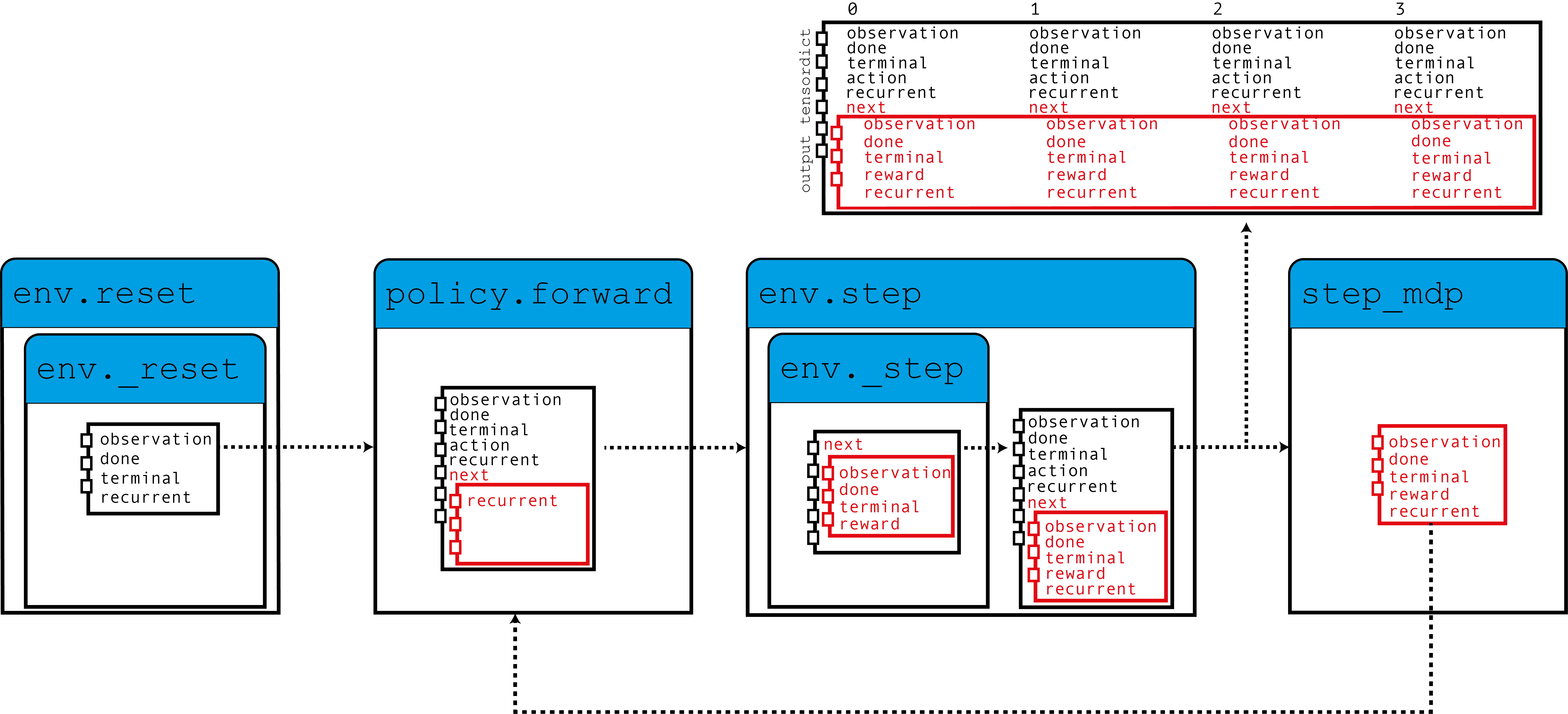
如圖所示，我們的環境用歸零的遞迴狀態填充 TensorDict，策略會讀取這些狀態以及觀測結果以產生動作，以及將用於下一步的遞迴狀態。當呼叫 step_mdp() 函數時，來自下一個狀態的遞迴狀態會被帶到當前的 TensorDict。讓我們看看這在實踐中是如何實現的。

如果您在 Google Colab 中運行此程式，請確保您安裝以下依賴項

!pip3 install torchrl
!pip3 install gym[mujoco]
!pip3 install tqdm

設定¶

import torch
import tqdm
from tensordict.nn import TensorDictModule as Mod, TensorDictSequential as Seq
from torch import nn
from torchrl.collectors import SyncDataCollector
from torchrl.data import LazyMemmapStorage, TensorDictReplayBuffer
from torchrl.envs import (
    Compose,
    ExplorationType,
    GrayScale,
    InitTracker,
    ObservationNorm,
    Resize,
    RewardScaling,
    set_exploration_type,
    StepCounter,
    ToTensorImage,
    TransformedEnv,
)
from torchrl.envs.libs.gym import GymEnv
from torchrl.modules import ConvNet, EGreedyModule, LSTMModule, MLP, QValueModule
from torchrl.objectives import DQNLoss, SoftUpdate

is_fork = multiprocessing.get_start_method() == "fork"
device = (
    torch.device(0)
    if torch.cuda.is_available() and not is_fork
    else torch.device("cpu")
)

環境¶

與往常一樣，第一步是建立我們的環境：它有助於我們定義問題並相應地建立策略網路。在本教學中，我們將運行 CartPole gym 環境的單個基於像素的實例，並帶有一些自定義轉換：轉換為灰度、調整大小為 84x84、縮小獎勵以及正規化觀測結果。

注意

StepCounter 轉換是輔助的。由於 CartPole 任務的目標是使軌跡盡可能長，因此計算步數可以幫助我們追蹤策略的效能。

對於本教學的目的，有兩個轉換非常重要

InitTracker 將透過在 TensorDict 中添加一個 "is_init" 布林遮罩來標記對 reset() 的呼叫，該遮罩將追蹤哪些步驟需要重設 RNN 隱藏狀態。
TensorDictPrimer 轉換有點技術性。使用 RNN 策略不需要它。但是，它會指示環境（以及隨後的收集器）預期會有額外的金鑰。一旦添加，對 env.reset() 的呼叫將使用歸零的張量填充在 primer 中指示的條目。知道這些張量是策略所預期的，收集器將在收集期間將它們傳遞下去。最終，我們將把隱藏狀態儲存在重播緩衝區中，這將有助於我們引導損失模組中 RNN 運算的計算（否則將以 0 啟動）。總而言之：不包含此轉換不會對我們策略的訓練產生巨大影響，但它會使遞迴金鑰從收集到的資料和重播緩衝區中消失，這反過來會導致稍微不那麼最佳的訓練。幸運的是，我們建議的 LSTMModule 配備了一個輔助方法，可以為我們建立該轉換，因此我們可以等到我們建立它！

env = TransformedEnv(
    GymEnv("CartPole-v1", from_pixels=True, device=device),
    Compose(
        ToTensorImage(),
        GrayScale(),
        Resize(84, 84),
        StepCounter(),
        InitTracker(),
        RewardScaling(loc=0.0, scale=0.1),
        ObservationNorm(standard_normal=True, in_keys=["pixels"]),
    ),
)

與往常一樣，我們需要手動初始化我們的正規化常數

env.transform[-1].init_stats(1000, reduce_dim=[0, 1, 2], cat_dim=0, keep_dims=[0])
td = env.reset()

策略¶

我們的策略將包含 3 個組成部分：一個 ConvNet 主幹網路、一個 LSTMModule 記憶層和一個淺層 MLP 區塊，用於將 LSTM 輸出映射到動作值。

卷積網路¶

我們構建了一個卷積網路，兩側是 torch.nn.AdaptiveAvgPool2d，它將把輸出壓縮成一個大小為 64 的向量。ConvNet 可以協助我們完成此操作

feature = Mod(
    ConvNet(
        num_cells=[32, 32, 64],
        squeeze_output=True,
        aggregator_class=nn.AdaptiveAvgPool2d,
        aggregator_kwargs={"output_size": (1, 1)},
        device=device,
    ),
    in_keys=["pixels"],
    out_keys=["embed"],
)

我們在批次資料上執行第一個模組，以收集輸出向量的大小

n_cells = feature(env.reset())["embed"].shape[-1]

LSTM 模組¶

TorchRL 提供了一個專用的 LSTMModule 類，用於將 LSTM 整合到您的程式碼庫中。它是一個 TensorDictModuleBase 子類：因此，它有一組 in_keys 和 out_keys，指示在模組執行期間應預期讀取和寫入/更新哪些值。該類別帶有可自訂的預定義值，用於這些屬性，以方便其構建。

注意

使用限制：該類別支援幾乎所有 LSTM 功能，例如 dropout 或多層 LSTM。但是，為了遵守 TorchRL 的慣例，此 LSTM 必須將 batch_first 屬性設定為 True，這不是 PyTorch 中的預設值。但是，我們的 LSTMModule 更改了此預設行為，因此我們可以正常進行原生呼叫。

此外，LSTM 不能將 bidirectional 屬性設定為 True，因為這在線上設定中無法使用。在這種情況下，預設值是正確的。

lstm = LSTMModule(
    input_size=n_cells,
    hidden_size=128,
    device=device,
    in_key="embed",
    out_key="embed",
)

讓我們看一下 LSTM 模組類別，特別是它的 in 和 out_keys

print("in_keys", lstm.in_keys)
print("out_keys", lstm.out_keys)

in_keys ['embed', 'recurrent_state_h', 'recurrent_state_c', 'is_init']
out_keys ['embed', ('next', 'recurrent_state_h'), ('next', 'recurrent_state_c')]

我們可以發現這些值包含我們指示為 in_key（和 out_key）的鍵以及循環鍵名稱。out_keys 前面有一個“next”字首，表示它們需要寫入“next”TensorDict。我們使用此慣例（可以透過傳遞 in_keys/out_keys 參數來覆蓋），以確保呼叫 step_mdp() 會將循環狀態移動到根 TensorDict，使其在後續呼叫期間可用於 RNN（請參閱簡介中的圖）。

如前所述，我們還有一個可選的轉換要添加到我們的環境中，以確保循環狀態傳遞到緩衝區。make_tensordict_primer() 方法完全做到了這一點

env.append_transform(lstm.make_tensordict_primer())

TransformedEnv(
    env=GymEnv(env=CartPole-v1, batch_size=torch.Size([]), device=cuda:0),
    transform=Compose(
            ToTensorImage(keys=['pixels']),
            GrayScale(keys=['pixels']),
            Resize(w=84, h=84, interpolation=InterpolationMode.BILINEAR, keys=['pixels']),
            StepCounter(keys=[]),
            InitTracker(keys=[]),
            RewardScaling(loc=0.0000, scale=0.1000, keys=['reward']),
            ObservationNorm(keys=['pixels']),
            TensorDictPrimer(primers=Composite(
                recurrent_state_h: UnboundedContinuous(
                    shape=torch.Size([1, 128]),
                    space=ContinuousBox(
                        low=Tensor(shape=torch.Size([1, 128]), device=cuda:0, dtype=torch.float32, contiguous=True),
                        high=Tensor(shape=torch.Size([1, 128]), device=cuda:0, dtype=torch.float32, contiguous=True)),
                    device=cuda:0,
                    dtype=torch.float32,
                    domain=continuous),
                recurrent_state_c: UnboundedContinuous(
                    shape=torch.Size([1, 128]),
                    space=ContinuousBox(
                        low=Tensor(shape=torch.Size([1, 128]), device=cuda:0, dtype=torch.float32, contiguous=True),
                        high=Tensor(shape=torch.Size([1, 128]), device=cuda:0, dtype=torch.float32, contiguous=True)),
                    device=cuda:0,
                    dtype=torch.float32,
                    domain=continuous),
                device=cuda:0,
                shape=torch.Size([])), default_value={'recurrent_state_h': 0.0, 'recurrent_state_c': 0.0}, random=None)))

就是這樣！我們可以列印環境以檢查一切是否正常，現在我們已經添加了 primer

print(env)

TransformedEnv(
    env=GymEnv(env=CartPole-v1, batch_size=torch.Size([]), device=cuda:0),
    transform=Compose(
            ToTensorImage(keys=['pixels']),
            GrayScale(keys=['pixels']),
            Resize(w=84, h=84, interpolation=InterpolationMode.BILINEAR, keys=['pixels']),
            StepCounter(keys=[]),
            InitTracker(keys=[]),
            RewardScaling(loc=0.0000, scale=0.1000, keys=['reward']),
            ObservationNorm(keys=['pixels']),
            TensorDictPrimer(primers=Composite(
                recurrent_state_h: UnboundedContinuous(
                    shape=torch.Size([1, 128]),
                    space=ContinuousBox(
                        low=Tensor(shape=torch.Size([1, 128]), device=cuda:0, dtype=torch.float32, contiguous=True),
                        high=Tensor(shape=torch.Size([1, 128]), device=cuda:0, dtype=torch.float32, contiguous=True)),
                    device=cuda:0,
                    dtype=torch.float32,
                    domain=continuous),
                recurrent_state_c: UnboundedContinuous(
                    shape=torch.Size([1, 128]),
                    space=ContinuousBox(
                        low=Tensor(shape=torch.Size([1, 128]), device=cuda:0, dtype=torch.float32, contiguous=True),
                        high=Tensor(shape=torch.Size([1, 128]), device=cuda:0, dtype=torch.float32, contiguous=True)),
                    device=cuda:0,
                    dtype=torch.float32,
                    domain=continuous),
                device=cuda:0,
                shape=torch.Size([])), default_value={'recurrent_state_h': 0.0, 'recurrent_state_c': 0.0}, random=None)))

MLP¶

我們使用單層 MLP 來表示將用於我們策略的動作值。

mlp = MLP(
    out_features=2,
    num_cells=[
        64,
    ],
    device=device,
)

並用零填充偏差

mlp[-1].bias.data.fill_(0.0)
mlp = Mod(mlp, in_keys=["embed"], out_keys=["action_value"])

使用 Q 值選擇動作¶

我們策略的最後一部分是 Q 值模組。Q 值模組 QValueModule 將讀取由我們的 MLP 產生的 "action_values" 鍵，並從中收集具有最大值的動作。我們唯一需要做的就是指定動作空間，可以透過傳遞字串或動作規範來完成。這使我們可以使用分類（有時稱為「稀疏」）編碼或其 one-hot 版本。

qval = QValueModule(spec=env.action_spec)

注意

TorchRL 還提供了一個封裝器類別 torchrl.modules.QValueActor，它將模組與 QValueModule 一起封裝在 Sequential 中，就像我們在此處明確地做的那樣。這樣做沒有什麼優勢，而且過程不太透明，但最終結果將與我們在此處所做的相似。

我們現在可以將所有內容放在一個 TensorDictSequential 中

stoch_policy = Seq(feature, lstm, mlp, qval)

DQN 是一種確定性演算法，探索是其中至關重要的部分。我們將使用一個 \(\epsilon\)-greedy 策略，其 epsilon 為 0.2，逐漸衰減到 0。這種衰減是透過呼叫 step() 來實現的（請參閱下面的訓練迴圈）。

exploration_module = EGreedyModule(
    annealing_num_steps=1_000_000, spec=env.action_spec, eps_init=0.2
)
stoch_policy = Seq(
    stoch_policy,
    exploration_module,
)

使用模型進行損失¶

我們建立的模型非常適合在序列設定中使用。但是，類別 torch.nn.LSTM 可以使用 cuDNN 優化的後端來更快地在 GPU 裝置上執行 RNN 序列。我們不想錯過這樣一個加速訓練迴圈的機會！要使用它，我們只需要告訴 LSTM 模組在使用損失時以「循環模式」執行。由於我們通常希望擁有 LSTM 模組的兩個副本，因此我們透過呼叫 set_recurrent_mode() 方法來做到這一點，該方法將傳回一個新的 LSTM 實例（具有共享權重），該實例將假定輸入資料本質上是序列的。

policy = Seq(feature, lstm.set_recurrent_mode(True), mlp, qval)

因為我們還有幾個未初始化的參數，所以我們應該在建立最佳化器之前先初始化它們。

policy(env.reset())

TensorDict(
    fields={
        action: Tensor(shape=torch.Size([2]), device=cuda:0, dtype=torch.int64, is_shared=True),
        action_value: Tensor(shape=torch.Size([2]), device=cuda:0, dtype=torch.float32, is_shared=True),
        chosen_action_value: Tensor(shape=torch.Size([1]), device=cuda:0, dtype=torch.float32, is_shared=True),
        done: Tensor(shape=torch.Size([1]), device=cuda:0, dtype=torch.bool, is_shared=True),
        embed: Tensor(shape=torch.Size([128]), device=cuda:0, dtype=torch.float32, is_shared=True),
        is_init: Tensor(shape=torch.Size([1]), device=cuda:0, dtype=torch.bool, is_shared=True),
        next: TensorDict(
            fields={
                recurrent_state_c: Tensor(shape=torch.Size([1, 128]), device=cuda:0, dtype=torch.float32, is_shared=True),
                recurrent_state_h: Tensor(shape=torch.Size([1, 128]), device=cuda:0, dtype=torch.float32, is_shared=True)},
            batch_size=torch.Size([]),
            device=cuda:0,
            is_shared=True),
        pixels: Tensor(shape=torch.Size([1, 84, 84]), device=cuda:0, dtype=torch.float32, is_shared=True),
        recurrent_state_c: Tensor(shape=torch.Size([1, 128]), device=cuda:0, dtype=torch.float32, is_shared=True),
        recurrent_state_h: Tensor(shape=torch.Size([1, 128]), device=cuda:0, dtype=torch.float32, is_shared=True),
        step_count: Tensor(shape=torch.Size([1]), device=cuda:0, dtype=torch.int64, is_shared=True),
        terminated: Tensor(shape=torch.Size([1]), device=cuda:0, dtype=torch.bool, is_shared=True),
        truncated: Tensor(shape=torch.Size([1]), device=cuda:0, dtype=torch.bool, is_shared=True)},
    batch_size=torch.Size([]),
    device=cuda:0,
    is_shared=True)

DQN 損失¶

我們的 DQN 損失要求我們傳遞策略，再次傳遞動作空間。雖然這看起來很多餘，但這很重要，因為我們希望確保 DQNLoss 和 QValueModule 類別是相容的，但彼此沒有強烈的依賴關係。

要使用 Double-DQN，我們要求一個 delay_value 參數，該參數將建立網路參數的非可微分副本，以用作目標網路。

loss_fn = DQNLoss(policy, action_space=env.action_spec, delay_value=True)

由於我們正在使用 double DQN，因此我們需要更新目標參數。我們將使用 SoftUpdate 實例來執行此工作。

updater = SoftUpdate(loss_fn, eps=0.95)

optim = torch.optim.Adam(policy.parameters(), lr=3e-4)

收集器和重播緩衝區¶

我們建立最簡單的資料收集器。我們將嘗試使用一百萬幀來訓練我們的演算法，一次擴展緩衝區 50 幀。緩衝區將被設計為儲存 20,000 個每個 50 步的軌跡。在每個最佳化步驟（每次資料收集 16 個）中，我們將從緩衝區中收集 4 個項目，總共 200 個轉換。我們將使用 LazyMemmapStorage 儲存體將資料保留在磁碟上。

注意

為了提高效率，我們僅在此處執行幾千次迭代。在實際設定中，幀總數應設定為 1M。

collector = SyncDataCollector(env, stoch_policy, frames_per_batch=50, total_frames=200, device=device)
rb = TensorDictReplayBuffer(
    storage=LazyMemmapStorage(20_000), batch_size=4, prefetch=10
)

訓練迴圈¶

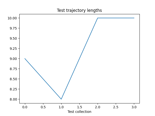
為了追蹤進度，我們將每 50 次資料收集在環境中執行一次策略，並在訓練後繪製結果。

utd = 16
pbar = tqdm.tqdm(total=1_000_000)
longest = 0

traj_lens = []
for i, data in enumerate(collector):
    if i == 0:
        print(
            "Let us print the first batch of data.\nPay attention to the key names "
            "which will reflect what can be found in this data structure, in particular: "
            "the output of the QValueModule (action_values, action and chosen_action_value),"
            "the 'is_init' key that will tell us if a step is initial or not, and the "
            "recurrent_state keys.\n",
            data,
        )
    pbar.update(data.numel())
    # it is important to pass data that is not flattened
    rb.extend(data.unsqueeze(0).to_tensordict().cpu())
    for _ in range(utd):
        s = rb.sample().to(device, non_blocking=True)
        loss_vals = loss_fn(s)
        loss_vals["loss"].backward()
        optim.step()
        optim.zero_grad()
    longest = max(longest, data["step_count"].max().item())
    pbar.set_description(
        f"steps: {longest}, loss_val: {loss_vals['loss'].item(): 4.4f}, action_spread: {data['action'].sum(0)}"
    )
    exploration_module.step(data.numel())
    updater.step()

    with set_exploration_type(ExplorationType.DETERMINISTIC), torch.no_grad():
        rollout = env.rollout(10000, stoch_policy)
        traj_lens.append(rollout.get(("next", "step_count")).max().item())

  0%|          | 0/1000000 [00:00<?, ?it/s]Let us print the first batch of data.
Pay attention to the key names which will reflect what can be found in this data structure, in particular: the output of the QValueModule (action_values, action and chosen_action_value),the 'is_init' key that will tell us if a step is initial or not, and the recurrent_state keys.
 TensorDict(
    fields={
        action: Tensor(shape=torch.Size([50, 2]), device=cuda:0, dtype=torch.int64, is_shared=True),
        action_value: Tensor(shape=torch.Size([50, 2]), device=cuda:0, dtype=torch.float32, is_shared=True),
        chosen_action_value: Tensor(shape=torch.Size([50, 1]), device=cuda:0, dtype=torch.float32, is_shared=True),
        collector: TensorDict(
            fields={
                traj_ids: Tensor(shape=torch.Size([50]), device=cuda:0, dtype=torch.int64, is_shared=True)},
            batch_size=torch.Size([50]),
            device=cuda:0,
            is_shared=True),
        done: Tensor(shape=torch.Size([50, 1]), device=cuda:0, dtype=torch.bool, is_shared=True),
        embed: Tensor(shape=torch.Size([50, 128]), device=cuda:0, dtype=torch.float32, is_shared=True),
        is_init: Tensor(shape=torch.Size([50, 1]), device=cuda:0, dtype=torch.bool, is_shared=True),
        next: TensorDict(
            fields={
                done: Tensor(shape=torch.Size([50, 1]), device=cuda:0, dtype=torch.bool, is_shared=True),
                is_init: Tensor(shape=torch.Size([50, 1]), device=cuda:0, dtype=torch.bool, is_shared=True),
                pixels: Tensor(shape=torch.Size([50, 1, 84, 84]), device=cuda:0, dtype=torch.float32, is_shared=True),
                recurrent_state_c: Tensor(shape=torch.Size([50, 1, 128]), device=cuda:0, dtype=torch.float32, is_shared=True),
                recurrent_state_h: Tensor(shape=torch.Size([50, 1, 128]), device=cuda:0, dtype=torch.float32, is_shared=True),
                reward: Tensor(shape=torch.Size([50, 1]), device=cuda:0, dtype=torch.float32, is_shared=True),
                step_count: Tensor(shape=torch.Size([50, 1]), device=cuda:0, dtype=torch.int64, is_shared=True),
                terminated: Tensor(shape=torch.Size([50, 1]), device=cuda:0, dtype=torch.bool, is_shared=True),
                truncated: Tensor(shape=torch.Size([50, 1]), device=cuda:0, dtype=torch.bool, is_shared=True)},
            batch_size=torch.Size([50]),
            device=cuda:0,
            is_shared=True),
        pixels: Tensor(shape=torch.Size([50, 1, 84, 84]), device=cuda:0, dtype=torch.float32, is_shared=True),
        recurrent_state_c: Tensor(shape=torch.Size([50, 1, 128]), device=cuda:0, dtype=torch.float32, is_shared=True),
        recurrent_state_h: Tensor(shape=torch.Size([50, 1, 128]), device=cuda:0, dtype=torch.float32, is_shared=True),
        step_count: Tensor(shape=torch.Size([50, 1]), device=cuda:0, dtype=torch.int64, is_shared=True),
        terminated: Tensor(shape=torch.Size([50, 1]), device=cuda:0, dtype=torch.bool, is_shared=True),
        truncated: Tensor(shape=torch.Size([50, 1]), device=cuda:0, dtype=torch.bool, is_shared=True)},
    batch_size=torch.Size([50]),
    device=cuda:0,
    is_shared=True)

  0%|          | 50/1000000 [00:00<1:27:22, 190.76it/s]
steps: 12, loss_val:  0.0004, action_spread: tensor([47,  3], device='cuda:0'):   0%|          | 50/1000000 [00:01<1:27:22, 190.76it/s]
steps: 12, loss_val:  0.0004, action_spread: tensor([47,  3], device='cuda:0'):   0%|          | 100/1000000 [00:01<5:16:29, 52.66it/s]
steps: 12, loss_val:  0.0003, action_spread: tensor([46,  4], device='cuda:0'):   0%|          | 100/1000000 [00:02<5:16:29, 52.66it/s]
steps: 12, loss_val:  0.0003, action_spread: tensor([46,  4], device='cuda:0'):   0%|          | 150/1000000 [00:02<5:43:36, 48.50it/s]
steps: 12, loss_val:  0.0002, action_spread: tensor([44,  6], device='cuda:0'):   0%|          | 150/1000000 [00:03<5:43:36, 48.50it/s]
steps: 12, loss_val:  0.0002, action_spread: tensor([44,  6], device='cuda:0'):   0%|          | 200/1000000 [00:04<6:04:34, 45.71it/s]
steps: 19, loss_val:  0.0002, action_spread: tensor([ 6, 44], device='cuda:0'):   0%|          | 200/1000000 [00:04<6:04:34, 45.71it/s]

讓我們繪製我們的結果

if traj_lens:
    from matplotlib import pyplot as plt

    plt.plot(traj_lens)
    plt.xlabel("Test collection")
    plt.title("Test trajectory lengths")

結論¶

我們已經了解如何在 TorchRL 的策略中加入 RNN。現在您應該能夠：

建立一個作為 TensorDictModule 的 LSTM 模組
透過 InitTracker 轉換，向 LSTM 模組指示需要重置
將此模組納入策略和損失模組中
確保收集器 (Collector) 知道循環狀態條目 (recurrent state entries)，以便它們可以與其餘資料一起儲存在重播緩衝區 (replay buffer) 中

延伸閱讀¶

TorchRL 的文件可以在這裡找到。

腳本總執行時間： ( 0 分鐘 9.009 秒)

由 Sphinx-Gallery 產生