PyTorch Numeric Suite 教學課程

建立於：2020 年 7 月 28 日 | 最後更新：2024 年 1 月 16 日 | 最後驗證：未驗證

簡介

量化在運作時很好，但當它不能滿足我們期望的準確度時，很難知道哪裡出錯。除錯量化的準確度問題並不容易且耗時。

除錯的一個重要步驟是測量浮點模型及其對應的量化模型的統計資料，以了解它們在哪裡差異最大。我們在 PyTorch 量化中建立了一套名為 PyTorch Numeric Suite 的數值工具，以支援量化模組和浮點模組之間的統計資料測量，以支援量化除錯工作。即使對於具有良好準確度的量化模型，PyTorch Numeric Suite 仍然可以用作分析工具，以更好地了解模型中的量化錯誤，並為進一步最佳化提供指導。

PyTorch Numeric Suite 目前支援透過靜態量化和動態量化量化的模型，並具有統一的 API。

在本教學課程中，我們將首先使用 ResNet18 作為範例，展示如何使用 PyTorch Numeric Suite 來測量 eager 模式中靜態量化模型和浮點模型之間的統計資料。然後，我們將使用基於 LSTM 的序列模型作為範例，展示 PyTorch Numeric Suite 用於動態量化模型的使用方式。

靜態量化的 Numeric Suite

設定

我們將從進行必要的匯入開始

import numpy as np
import torch
import torch.nn as nn
import torchvision
from torchvision import models, datasets
import torchvision.transforms as transforms
import os
import torch.quantization
import torch.quantization._numeric_suite as ns
from torch.quantization import (
    default_eval_fn,
    default_qconfig,
    quantize,
)

然後我們載入預先訓練的浮點 ResNet18 模型，並將其量化為 qmodel。我們無法比較兩個任意模型，只能比較浮點模型和從它衍生的量化模型。

float_model = torchvision.models.quantization.resnet18(weights=models.ResNet18_Weights.IMAGENET1K_V1, quantize=False)
float_model.to('cpu')
float_model.eval()
float_model.fuse_model()
float_model.qconfig = torch.quantization.default_qconfig
img_data = [(torch.rand(2, 3, 10, 10, dtype=torch.float), torch.randint(0, 1, (2,), dtype=torch.long)) for _ in range(2)]
qmodel = quantize(float_model, default_eval_fn, [img_data], inplace=False)

Downloading: "https://download.pytorch.org/models/resnet18-f37072fd.pth" to /var/lib/ci-user/.cache/torch/hub/checkpoints/resnet18-f37072fd.pth


  0%|          | 0.00/44.7M [00:00<?, ?B/s]

 46%|####6     | 20.8M/44.7M [00:00<00:00, 217MB/s]

 94%|#########4| 42.1M/44.7M [00:00<00:00, 221MB/s]
100%|##########| 44.7M/44.7M [00:00<00:00, 220MB/s]

1. 比較浮點模型和量化模型的權重

我們通常要比較的第一件事是量化模型和浮點模型的權重。我們可以從 PyTorch Numeric Suite 呼叫 compare_weights() 來取得字典 wt_compare_dict，其中鍵對應於模組名稱，每個條目都是一個字典，其中包含兩個鍵 'float' 和 'quantized'，分別包含浮點權重和量化權重。compare_weights() 接收浮點和量化狀態字典，並傳回一個字典，其鍵對應於浮點權重，值是浮點權重和量化權重的字典

wt_compare_dict = ns.compare_weights(float_model.state_dict(), qmodel.state_dict())

print('keys of wt_compare_dict:')
print(wt_compare_dict.keys())

print("\nkeys of wt_compare_dict entry for conv1's weight:")
print(wt_compare_dict['conv1.weight'].keys())
print(wt_compare_dict['conv1.weight']['float'].shape)
print(wt_compare_dict['conv1.weight']['quantized'].shape)

keys of wt_compare_dict:
dict_keys(['conv1.weight', 'layer1.0.conv1.weight', 'layer1.0.conv2.weight', 'layer1.1.conv1.weight', 'layer1.1.conv2.weight', 'layer2.0.conv1.weight', 'layer2.0.conv2.weight', 'layer2.0.downsample.0.weight', 'layer2.1.conv1.weight', 'layer2.1.conv2.weight', 'layer3.0.conv1.weight', 'layer3.0.conv2.weight', 'layer3.0.downsample.0.weight', 'layer3.1.conv1.weight', 'layer3.1.conv2.weight', 'layer4.0.conv1.weight', 'layer4.0.conv2.weight', 'layer4.0.downsample.0.weight', 'layer4.1.conv1.weight', 'layer4.1.conv2.weight', 'fc._packed_params._packed_params'])

keys of wt_compare_dict entry for conv1's weight:
dict_keys(['float', 'quantized'])
torch.Size([64, 3, 7, 7])
torch.Size([64, 3, 7, 7])

一旦取得 wt_compare_dict，使用者可以以他們想要的任何方式處理這個字典。這裡作為一個例子，我們計算浮點模型和量化模型的權重的量化誤差如下。計算量化張量 y 的訊號量化雜訊比 (SQNR)。SQNR 反映了最大標稱訊號強度與量化中引入的量化誤差之間的關係。較高的 SQNR 對應於較低的量化誤差。

def compute_error(x, y):
    Ps = torch.norm(x)
    Pn = torch.norm(x-y)
    return 20*torch.log10(Ps/Pn)

for key in wt_compare_dict:
    print(key, compute_error(wt_compare_dict[key]['float'], wt_compare_dict[key]['quantized'].dequantize()))

conv1.weight tensor(31.6638)
layer1.0.conv1.weight tensor(30.6450)
layer1.0.conv2.weight tensor(31.1528)
layer1.1.conv1.weight tensor(32.1438)
layer1.1.conv2.weight tensor(31.2477)
layer2.0.conv1.weight tensor(30.9890)
layer2.0.conv2.weight tensor(28.8233)
layer2.0.downsample.0.weight tensor(31.5558)
layer2.1.conv1.weight tensor(30.7668)
layer2.1.conv2.weight tensor(28.4516)
layer3.0.conv1.weight tensor(30.9247)
layer3.0.conv2.weight tensor(26.6841)
layer3.0.downsample.0.weight tensor(28.7825)
layer3.1.conv1.weight tensor(28.9707)
layer3.1.conv2.weight tensor(25.6784)
layer4.0.conv1.weight tensor(26.8495)
layer4.0.conv2.weight tensor(25.8394)
layer4.0.downsample.0.weight tensor(28.6355)
layer4.1.conv1.weight tensor(26.8758)
layer4.1.conv2.weight tensor(28.4319)
fc._packed_params._packed_params tensor(32.6505)

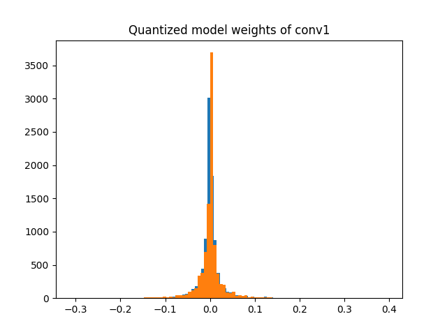
作為另一個範例，wt_compare_dict 也可以用於繪製浮點模型和量化模型的權重的直方圖。

import matplotlib.pyplot as plt

f = wt_compare_dict['conv1.weight']['float'].flatten()
plt.hist(f, bins = 100)
plt.title("Floating point model weights of conv1")
plt.show()

q = wt_compare_dict['conv1.weight']['quantized'].flatten().dequantize()
plt.hist(q, bins = 100)
plt.title("Quantized model weights of conv1")
plt.show()

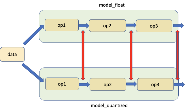
2. 比較相應位置的浮點模型和量化模型

第二個工具允許比較相同輸入的浮點模型和量化模型之間相應位置的權重和激活，如下圖所示。紅色箭頭表示比較的位置。

我們從 PyTorch Numeric Suite 呼叫 compare_model_outputs() 來取得給定輸入資料的浮點模型和量化模型中相應位置的激活。此 API 傳回一個字典，其中模組名稱為鍵。每個條目本身是一個字典，其中包含兩個鍵 'float' 和 'quantized'，分別包含激活。

data = img_data[0][0]

# Take in floating point and quantized model as well as input data, and returns a dict, with keys
# corresponding to the quantized module names and each entry being a dictionary with two keys 'float' and
# 'quantized', containing the activations of floating point and quantized model at matching locations.
act_compare_dict = ns.compare_model_outputs(float_model, qmodel, data)

print('keys of act_compare_dict:')
print(act_compare_dict.keys())

print("\nkeys of act_compare_dict entry for conv1's output:")
print(act_compare_dict['conv1.stats'].keys())
print(act_compare_dict['conv1.stats']['float'][0].shape)
print(act_compare_dict['conv1.stats']['quantized'][0].shape)

keys of act_compare_dict:
dict_keys(['conv1.stats', 'layer1.0.conv1.stats', 'layer1.0.conv2.stats', 'layer1.0.add_relu.stats', 'layer1.1.conv1.stats', 'layer1.1.conv2.stats', 'layer1.1.add_relu.stats', 'layer2.0.conv1.stats', 'layer2.0.conv2.stats', 'layer2.0.downsample.0.stats', 'layer2.0.add_relu.stats', 'layer2.1.conv1.stats', 'layer2.1.conv2.stats', 'layer2.1.add_relu.stats', 'layer3.0.conv1.stats', 'layer3.0.conv2.stats', 'layer3.0.downsample.0.stats', 'layer3.0.add_relu.stats', 'layer3.1.conv1.stats', 'layer3.1.conv2.stats', 'layer3.1.add_relu.stats', 'layer4.0.conv1.stats', 'layer4.0.conv2.stats', 'layer4.0.downsample.0.stats', 'layer4.0.add_relu.stats', 'layer4.1.conv1.stats', 'layer4.1.conv2.stats', 'layer4.1.add_relu.stats', 'fc.stats', 'quant.stats'])

keys of act_compare_dict entry for conv1's output:
dict_keys(['float', 'quantized'])
torch.Size([2, 64, 5, 5])
torch.Size([2, 64, 5, 5])

這個字典可用於比較和計算浮點模型和量化模型的激活的量化誤差，如下所示。

for key in act_compare_dict:
    print(key, compute_error(act_compare_dict[key]['float'][0], act_compare_dict[key]['quantized'][0].dequantize()))

conv1.stats tensor(37.1388, grad_fn=<MulBackward0>)
layer1.0.conv1.stats tensor(30.1562, grad_fn=<MulBackward0>)
layer1.0.conv2.stats tensor(29.0511, grad_fn=<MulBackward0>)
layer1.0.add_relu.stats tensor(32.7605, grad_fn=<MulBackward0>)
layer1.1.conv1.stats tensor(30.1330, grad_fn=<MulBackward0>)
layer1.1.conv2.stats tensor(26.3872, grad_fn=<MulBackward0>)
layer1.1.add_relu.stats tensor(30.0649, grad_fn=<MulBackward0>)
layer2.0.conv1.stats tensor(26.9528, grad_fn=<MulBackward0>)
layer2.0.conv2.stats tensor(26.7812, grad_fn=<MulBackward0>)
layer2.0.downsample.0.stats tensor(23.2544, grad_fn=<MulBackward0>)
layer2.0.add_relu.stats tensor(26.2048, grad_fn=<MulBackward0>)
layer2.1.conv1.stats tensor(25.6735, grad_fn=<MulBackward0>)
layer2.1.conv2.stats tensor(24.6564, grad_fn=<MulBackward0>)
layer2.1.add_relu.stats tensor(26.0816, grad_fn=<MulBackward0>)
layer3.0.conv1.stats tensor(26.9846, grad_fn=<MulBackward0>)
layer3.0.conv2.stats tensor(26.8694, grad_fn=<MulBackward0>)
layer3.0.downsample.0.stats tensor(25.1453, grad_fn=<MulBackward0>)
layer3.0.add_relu.stats tensor(24.8748, grad_fn=<MulBackward0>)
layer3.1.conv1.stats tensor(31.0022, grad_fn=<MulBackward0>)
layer3.1.conv2.stats tensor(26.1478, grad_fn=<MulBackward0>)
layer3.1.add_relu.stats tensor(25.5775, grad_fn=<MulBackward0>)
layer4.0.conv1.stats tensor(27.4940, grad_fn=<MulBackward0>)
layer4.0.conv2.stats tensor(27.2149, grad_fn=<MulBackward0>)
layer4.0.downsample.0.stats tensor(22.5105, grad_fn=<MulBackward0>)
layer4.0.add_relu.stats tensor(21.2105, grad_fn=<MulBackward0>)
layer4.1.conv1.stats tensor(26.5055, grad_fn=<MulBackward0>)
layer4.1.conv2.stats tensor(18.5702, grad_fn=<MulBackward0>)
layer4.1.add_relu.stats tensor(18.5091, grad_fn=<MulBackward0>)
fc.stats tensor(20.7117, grad_fn=<MulBackward0>)
quant.stats tensor(47.9043)

如果我們想要對多個輸入資料進行比較，我們可以執行以下操作。如果浮點模組和量化模組在 white_list 中，則透過將記錄器附加到浮點模組和量化模組來準備模型。預設記錄器為 OutputLogger，預設 white_list 為 DEFAULT_NUMERIC_SUITE_COMPARE_MODEL_OUTPUT_WHITE_LIST

ns.prepare_model_outputs(float_model, qmodel)

for data in img_data:
    float_model(data[0])
    qmodel(data[0])

# Find the matching activation between floating point and quantized modules, and return a dict with key
# corresponding to quantized module names and each entry being a dictionary with two keys 'float'
# and 'quantized', containing the matching floating point and quantized activations logged by the logger
act_compare_dict = ns.get_matching_activations(float_model, qmodel)

上述 API 中使用的預設日誌記錄器是 OutputLogger，它用於記錄模組的輸出。我們可以繼承基礎 Logger 類別，並建立我們自己的日誌記錄器來執行不同的功能。例如，我們可以建立一個新的 MyOutputLogger 類別，如下所示。

class MyOutputLogger(ns.Logger):
    r"""Customized logger class
    """

    def __init__(self):
        super(MyOutputLogger, self).__init__()

    def forward(self, x):
        # Custom functionalities
        # ...
        return x

然後我們可以將此日誌記錄器傳遞到上述 API 中，例如

data = img_data[0][0]
act_compare_dict = ns.compare_model_outputs(float_model, qmodel, data, logger_cls=MyOutputLogger)

或

ns.prepare_model_outputs(float_model, qmodel, MyOutputLogger)
for data in img_data:
    float_model(data[0])
    qmodel(data[0])
act_compare_dict = ns.get_matching_activations(float_model, qmodel)

3. 比較量化模型中的模組與其浮點等效模組，使用相同的輸入資料

第三個工具可以比較模型中的量化模組與其浮點對應物，將相同的輸入饋入兩者並比較它們的輸出，如下所示。

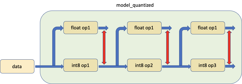
實際上，我們調用 prepare_model_with_stubs() 來替換我們想要與 Shadow 模組比較的量化模組，如下圖所示

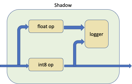
Shadow 模組將量化模組、浮點模組和日誌記錄器作為輸入，並在內部建立一個正向路徑，使浮點模組能夠共享相同的輸入張量來 Shadow 量化模組。

日誌記錄器是可以自訂的，預設日誌記錄器是 ShadowLogger，它將儲存量化模組和浮點模組的輸出，可用於計算模組級別的量化誤差。

請注意，在每次調用 compare_model_outputs() 和 compare_model_stub() 之前，我們需要有乾淨的浮點模型和量化模型。這是因為 compare_model_outputs() 和 compare_model_stub() 會就地修改浮點模型和量化模型，如果一個接一個地調用，將會導致意外的結果。

float_model = torchvision.models.quantization.resnet18(weights=models.ResNet18_Weights.IMAGENET1K_V1, quantize=False)
float_model.to('cpu')
float_model.eval()
float_model.fuse_model()
float_model.qconfig = torch.quantization.default_qconfig
img_data = [(torch.rand(2, 3, 10, 10, dtype=torch.float), torch.randint(0, 1, (2,), dtype=torch.long)) for _ in range(2)]
qmodel = quantize(float_model, default_eval_fn, [img_data], inplace=False)

在以下範例中，我們從 PyTorch Numeric Suite 調用 compare_model_stub()，以比較 QuantizableBasicBlock 模組與其浮點等效模組。此 API 返回一個字典，其鍵對應於模組名稱，每個條目都是一個字典，其中包含兩個鍵 'float' 和 'quantized'，其中包含量化模組及其匹配的浮點 Shadow 模組的輸出張量。

data = img_data[0][0]
module_swap_list = [torchvision.models.quantization.resnet.QuantizableBasicBlock]

# Takes in floating point and quantized model as well as input data, and returns a dict with key
# corresponding to module names and each entry being a dictionary with two keys 'float' and
# 'quantized', containing the output tensors of quantized module and its matching floating point shadow module.
ob_dict = ns.compare_model_stub(float_model, qmodel, module_swap_list, data)

print('keys of ob_dict:')
print(ob_dict.keys())

print("\nkeys of ob_dict entry for layer1.0's output:")
print(ob_dict['layer1.0.stats'].keys())
print(ob_dict['layer1.0.stats']['float'][0].shape)
print(ob_dict['layer1.0.stats']['quantized'][0].shape)

keys of ob_dict:
dict_keys(['layer1.0.stats', 'layer1.1.stats', 'layer2.0.stats', 'layer2.1.stats', 'layer3.0.stats', 'layer3.1.stats', 'layer4.0.stats', 'layer4.1.stats'])

keys of ob_dict entry for layer1.0's output:
dict_keys(['float', 'quantized'])
torch.Size([64, 3, 3])
torch.Size([64, 3, 3])

然後可以使用此字典來比較和計算模組級別的量化誤差。

for key in ob_dict:
    print(key, compute_error(ob_dict[key]['float'][0], ob_dict[key]['quantized'][0].dequantize()))

layer1.0.stats tensor(32.7203)
layer1.1.stats tensor(34.8070)
layer2.0.stats tensor(29.3657)
layer2.1.stats tensor(31.0864)
layer3.0.stats tensor(28.5980)
layer3.1.stats tensor(31.3857)
layer4.0.stats tensor(25.3010)
layer4.1.stats tensor(22.9801)

如果我們想要對多個輸入資料進行比較，我們可以執行以下操作。

ns.prepare_model_with_stubs(float_model, qmodel, module_swap_list, ns.ShadowLogger)
for data in img_data:
    qmodel(data[0])
ob_dict = ns.get_logger_dict(qmodel)

上述 API 中使用的預設日誌記錄器是 ShadowLogger，它用於記錄量化模組及其匹配的浮點 Shadow 模組的輸出。我們可以繼承基礎 Logger 類別，並建立我們自己的日誌記錄器來執行不同的功能。例如，我們可以建立一個新的 MyShadowLogger 類別，如下所示。

class MyShadowLogger(ns.Logger):
    r"""Customized logger class
    """

    def __init__(self):
        super(MyShadowLogger, self).__init__()

    def forward(self, x, y):
        # Custom functionalities
        # ...
        return x

然後我們可以將此日誌記錄器傳遞到上述 API 中，例如

data = img_data[0][0]
ob_dict = ns.compare_model_stub(float_model, qmodel, module_swap_list, data, logger_cls=MyShadowLogger)

或

ns.prepare_model_with_stubs(float_model, qmodel, module_swap_list, MyShadowLogger)
for data in img_data:
    qmodel(data[0])
ob_dict = ns.get_logger_dict(qmodel)

動態量化的 Numeric Suite

Numeric Suite API 的設計方式使其適用於動態量化模型和靜態量化模型。我們將使用具有 LSTM 和 Linear 模組的模型來演示 Numeric Suite 在動態量化模型上的用法。此模型與 LSTM 單詞語言模型 [1] 上的動態量化教程中使用的模型相同。

設定

首先，我們定義模型如下。請注意，在此模型中，只有 nn.LSTM 和 nn.Linear 模組將被動態量化，而 nn.Embedding 在量化後將保持為浮點模組。

class LSTMModel(nn.Module):
    """Container module with an encoder, a recurrent module, and a decoder."""

    def __init__(self, ntoken, ninp, nhid, nlayers, dropout=0.5):
        super(LSTMModel, self).__init__()
        self.encoder = nn.Embedding(ntoken, ninp)
        self.rnn = nn.LSTM(ninp, nhid, nlayers, dropout=dropout)
        self.decoder = nn.Linear(nhid, ntoken)

        self.init_weights()

        self.nhid = nhid
        self.nlayers = nlayers

    def init_weights(self):
        initrange = 0.1
        self.encoder.weight.data.uniform_(-initrange, initrange)
        self.decoder.bias.data.zero_()
        self.decoder.weight.data.uniform_(-initrange, initrange)

    def forward(self, input, hidden):
        emb = self.encoder(input)
        output, hidden = self.rnn(emb, hidden)
        decoded = self.decoder(output)
        return decoded, hidden

    def init_hidden(self, bsz):
        weight = next(self.parameters())
        return (weight.new_zeros(self.nlayers, bsz, self.nhid),
                weight.new_zeros(self.nlayers, bsz, self.nhid))

然後，我們建立 float_model 並將其量化為 qmodel。

ntokens = 10

float_model = LSTMModel(
    ntoken = ntokens,
    ninp = 512,
    nhid = 256,
    nlayers = 5,
)

float_model.eval()

qmodel = torch.quantization.quantize_dynamic(
    float_model, {nn.LSTM, nn.Linear}, dtype=torch.qint8
)

1. 比較浮點模型和量化模型的權重

我們首先從 PyTorch Numeric Suite 調用 compare_weights() 以取得字典 wt_compare_dict，其鍵對應於模組名稱，每個條目都是一個字典，其中包含兩個鍵 'float' 和 'quantized'，其中包含浮點權重和量化權重。

wt_compare_dict = ns.compare_weights(float_model.state_dict(), qmodel.state_dict())

一旦我們取得 wt_compare_dict，就可以使用它來比較和計算浮點模型和量化模型的權重的量化誤差，如下所示。

for key in wt_compare_dict:
    if wt_compare_dict[key]['quantized'].is_quantized:
        print(key, compute_error(wt_compare_dict[key]['float'], wt_compare_dict[key]['quantized'].dequantize()))
    else:
        print(key, compute_error(wt_compare_dict[key]['float'], wt_compare_dict[key]['quantized']))

encoder.weight tensor(inf)
rnn._all_weight_values.0.param tensor(48.1323)
rnn._all_weight_values.1.param tensor(48.1355)
rnn._all_weight_values.2.param tensor(48.1213)
rnn._all_weight_values.3.param tensor(48.1506)
rnn._all_weight_values.4.param tensor(48.1348)
decoder._packed_params._packed_params tensor(48.0233)

上面 encoder.weight 條目中的 Inf 值是因為編碼器模組未被量化，並且浮點模型和量化模型中的權重相同。

2. 比較相應位置的浮點模型和量化模型

然後，我們從 PyTorch Numeric Suite 調用 compare_model_outputs() 以取得給定輸入資料在相應位置的浮點模型和量化模型中的激活。此 API 返回一個字典，其中模組名稱是鍵。每個條目本身是一個字典，其中包含兩個鍵 'float' 和 'quantized'，其中包含激活。請注意，此序列模型有兩個輸入，我們可以將兩個輸入都傳遞到 compare_model_outputs() 和 compare_model_stub() 中。

input_ = torch.randint(ntokens, (1, 1), dtype=torch.long)
hidden = float_model.init_hidden(1)

act_compare_dict = ns.compare_model_outputs(float_model, qmodel, input_, hidden)
print(act_compare_dict.keys())

dict_keys(['encoder.stats', 'rnn.stats', 'decoder.stats'])

此字典可用於比較和計算浮點模型和量化模型的激活的量化誤差，如下所示。此模型中的 LSTM 模組有兩個輸出，在此範例中，我們計算第一個輸出的誤差。

for key in act_compare_dict:
    print(key, compute_error(act_compare_dict[key]['float'][0][0], act_compare_dict[key]['quantized'][0][0]))

encoder.stats tensor(inf, grad_fn=<MulBackward0>)
rnn.stats tensor(54.7745, grad_fn=<MulBackward0>)
decoder.stats tensor(37.2282, grad_fn=<MulBackward0>)

3. 比較量化模型中的模組與其浮點等效模組，使用相同的輸入資料

接下來，我們從 PyTorch Numeric Suite 調用 compare_model_stub() 以比較 LSTM 和 Linear 模組與其浮點等效模組。此 API 返回一個字典，其鍵對應於模組名稱，每個條目都是一個字典，其中包含兩個鍵 'float' 和 'quantized'，其中包含量化模組及其匹配的浮點 Shadow 模組的輸出張量。

我們先重置模型。

float_model = LSTMModel(
    ntoken = ntokens,
    ninp = 512,
    nhid = 256,
    nlayers = 5,
)
float_model.eval()

qmodel = torch.quantization.quantize_dynamic(
    float_model, {nn.LSTM, nn.Linear}, dtype=torch.qint8
)

接下來，我們從 PyTorch Numeric Suite 調用 compare_model_stub() 以比較 LSTM 和 Linear 模組與其浮點等效模組。此 API 返回一個字典，其鍵對應於模組名稱，每個條目都是一個字典，其中包含兩個鍵 'float' 和 'quantized'，其中包含量化模組及其匹配的浮點 Shadow 模組的輸出張量。

module_swap_list = [nn.Linear, nn.LSTM]
ob_dict = ns.compare_model_stub(float_model, qmodel, module_swap_list, input_, hidden)
print(ob_dict.keys())

dict_keys(['rnn.stats', 'decoder.stats'])

然後可以使用此字典來比較和計算模組級別的量化誤差。

for key in ob_dict:
    print(key, compute_error(ob_dict[key]['float'][0], ob_dict[key]['quantized'][0]))

rnn.stats tensor(54.6112)
decoder.stats tensor(40.2375)

40 dB 的 SQNR 很高，並且在這種情況下，浮點模型和量化模型之間具有非常好的數值對齊。

結論

在本教程中，我們演示了如何使用 PyTorch Numeric Suite 來測量和比較量化模型和浮點模型之間在 Eager 模式下的統計資訊，並且靜態量化和動態量化都使用統一的 API。

感謝您的閱讀！與往常一樣，我們歡迎任何回饋，因此如果您有任何問題，請在此處建立一個 Issue here。

參考文獻

[1] LSTM 單詞語言模型上的動態量化。