訓練分類器

建立於: 2017 年 3 月 24 日 | 最後更新: 2024 年 12 月 20 日 | 最後驗證: 未驗證

就是這樣。您已經了解如何定義神經網路、計算損失以及更新網路的權重。

現在您可能會想，

那資料呢？

通常，當您需要處理圖像、文字、音訊或影片資料時，可以使用標準的 Python 函式庫，將資料載入到 NumPy 陣列中。 然後，您可以將此陣列轉換為 torch.*Tensor。

• 對於圖像，Pillow、OpenCV 等函式庫很有用

• 對於音訊，scipy 和 librosa 等函式庫很有用

• 對於文字，可以使用原始 Python 或基於 Cython 的載入，或 NLTK 和 SpaCy 很有用

特別是對於視覺，我們建立了一個名為 torchvision 的函式庫，其中包含常用資料集（例如 ImageNet、CIFAR10、MNIST 等）的資料載入器和圖像的資料轉換器，即 torchvision.datasets 和 torch.utils.data.DataLoader。

這提供了極大的便利性，並避免了編寫樣板程式碼。

在本教學中，我們將使用 CIFAR10 資料集。 它有以下類別：「airplane」、「automobile」、「bird」、「cat」、「deer」、「dog」、「frog」、「horse」、「ship」、「truck」。 CIFAR-10 中的圖像大小為 3x32x32，即 3 個通道的 32x32 像素彩色圖像。

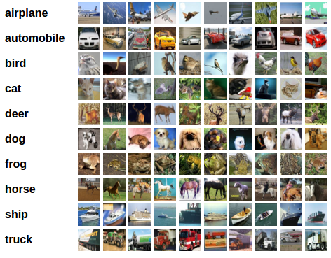
cifar10

訓練圖像分類器

我們將按以下步驟進行

1. 使用 torchvision 載入並正規化 CIFAR10 訓練和測試資料集

2. 定義卷積神經網路

3. 定義損失函數

4. 在訓練資料上訓練網路

5. 在測試資料上測試網路

1. 載入並正規化 CIFAR10

使用 torchvision，載入 CIFAR10 非常容易。

import torch
import torchvision
import torchvision.transforms as transforms

torchvision 資料集的輸出是範圍 [0, 1] 的 PILImage 圖像。 我們將它們轉換為正規化範圍 [-1, 1] 的張量。

注意

如果在 Windows 上執行並遇到 BrokenPipeError，請嘗試將 torch.utils.data.DataLoader() 的 num_worker 設為 0。

transform = transforms.Compose(
    [transforms.ToTensor(),
     transforms.Normalize((0.5, 0.5, 0.5), (0.5, 0.5, 0.5))])

batch_size = 4

trainset = torchvision.datasets.CIFAR10(root='./data', train=True,
                                        download=True, transform=transform)
trainloader = torch.utils.data.DataLoader(trainset, batch_size=batch_size,
                                          shuffle=True, num_workers=2)

testset = torchvision.datasets.CIFAR10(root='./data', train=False,
                                       download=True, transform=transform)
testloader = torch.utils.data.DataLoader(testset, batch_size=batch_size,
                                         shuffle=False, num_workers=2)

classes = ('plane', 'car', 'bird', 'cat',
           'deer', 'dog', 'frog', 'horse', 'ship', 'truck')

  0%|          | 0.00/170M [00:00<?, ?B/s]
  0%|          | 655k/170M [00:00<00:25, 6.54MB/s]
  5%|4         | 8.52M/170M [00:00<00:03, 48.9MB/s]
 11%|#1        | 19.1M/170M [00:00<00:02, 74.9MB/s]
 18%|#7        | 30.5M/170M [00:00<00:01, 90.4MB/s]
 24%|##4       | 41.3M/170M [00:00<00:01, 96.5MB/s]
 31%|###       | 52.4M/170M [00:00<00:01, 101MB/s]
 37%|###7      | 63.5M/170M [00:00<00:01, 104MB/s]
 43%|####3     | 74.2M/170M [00:00<00:00, 105MB/s]
 50%|####9     | 84.7M/170M [00:00<00:00, 105MB/s]
 56%|#####5    | 95.2M/170M [00:01<00:00, 104MB/s]
 62%|######2   | 106M/170M [00:01<00:00, 106MB/s]
 69%|######8   | 117M/170M [00:01<00:00, 107MB/s]
 75%|#######5  | 128M/170M [00:01<00:00, 107MB/s]
 82%|########1 | 139M/170M [00:01<00:00, 109MB/s]
 88%|########8 | 150M/170M [00:01<00:00, 108MB/s]
 95%|#########4| 162M/170M [00:01<00:00, 109MB/s]
100%|##########| 170M/170M [00:01<00:00, 101MB/s]

讓我們展示一些訓練圖像，供大家欣賞。

import matplotlib.pyplot as plt
import numpy as np

# functions to show an image


def imshow(img):
    img = img / 2 + 0.5     # unnormalize
    npimg = img.numpy()
    plt.imshow(np.transpose(npimg, (1, 2, 0)))
    plt.show()


# get some random training images
dataiter = iter(trainloader)
images, labels = next(dataiter)

# show images
imshow(torchvision.utils.make_grid(images))
# print labels
print(' '.join(f'{classes[labels[j]]:5s}' for j in range(batch_size)))

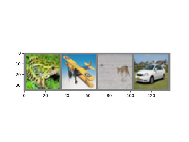
frog  plane deer  car

2. 定義卷積神經網路

從先前的神經網路部分複製神經網路，並修改它以採用 3 個通道的圖像 (而不是它定義的 1 個通道的圖像)。

import torch.nn as nn
import torch.nn.functional as F


class Net(nn.Module):
    def __init__(self):
        super().__init__()
        self.conv1 = nn.Conv2d(3, 6, 5)
        self.pool = nn.MaxPool2d(2, 2)
        self.conv2 = nn.Conv2d(6, 16, 5)
        self.fc1 = nn.Linear(16 * 5 * 5, 120)
        self.fc2 = nn.Linear(120, 84)
        self.fc3 = nn.Linear(84, 10)

    def forward(self, x):
        x = self.pool(F.relu(self.conv1(x)))
        x = self.pool(F.relu(self.conv2(x)))
        x = torch.flatten(x, 1) # flatten all dimensions except batch
        x = F.relu(self.fc1(x))
        x = F.relu(self.fc2(x))
        x = self.fc3(x)
        return x


net = Net()

3. 定義損失函數和最佳化器

讓我們使用分類交叉熵損失和帶動量的 SGD。

import torch.optim as optim

criterion = nn.CrossEntropyLoss()
optimizer = optim.SGD(net.parameters(), lr=0.001, momentum=0.9)

4. 訓練網路

當事情開始變得有趣時。 我們只需遍歷我們的資料迭代器，將輸入饋送到網路並進行最佳化。

for epoch in range(2):  # loop over the dataset multiple times

    running_loss = 0.0
    for i, data in enumerate(trainloader, 0):
        # get the inputs; data is a list of [inputs, labels]
        inputs, labels = data

        # zero the parameter gradients
        optimizer.zero_grad()

        # forward + backward + optimize
        outputs = net(inputs)
        loss = criterion(outputs, labels)
        loss.backward()
        optimizer.step()

        # print statistics
        running_loss += loss.item()
        if i % 2000 == 1999:    # print every 2000 mini-batches
            print(f'[{epoch + 1}, {i + 1:5d}] loss: {running_loss / 2000:.3f}')
            running_loss = 0.0

print('Finished Training')

[1,  2000] loss: 2.144
[1,  4000] loss: 1.835
[1,  6000] loss: 1.677
[1,  8000] loss: 1.573
[1, 10000] loss: 1.526
[1, 12000] loss: 1.447
[2,  2000] loss: 1.405
[2,  4000] loss: 1.363
[2,  6000] loss: 1.341
[2,  8000] loss: 1.340
[2, 10000] loss: 1.315
[2, 12000] loss: 1.281
Finished Training

讓我們快速儲存我們訓練好的模型

PATH = './cifar_net.pth'
torch.save(net.state_dict(), PATH)

有關儲存 PyTorch 模型的更多詳細資訊，請參閱此處。

5. 在測試資料上測試網路

我們已經針對訓練資料集進行了 2 次傳遞來訓練網路。 但我們需要檢查網路是否學到了任何東西。

我們將透過預測神經網路輸出的類別標籤並將其與實際情況進行比較來檢查這一點。 如果預測正確，我們會將樣本新增到正確預測的清單中。

好的，第一步。 讓我們顯示測試集中的圖像，以便熟悉一下。

dataiter = iter(testloader)
images, labels = next(dataiter)

# print images
imshow(torchvision.utils.make_grid(images))
print('GroundTruth: ', ' '.join(f'{classes[labels[j]]:5s}' for j in range(4)))

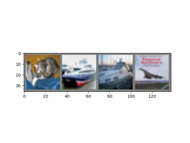
GroundTruth:  cat   ship  ship  plane

接下來，讓我們重新載入我們儲存的模型 (注意：這裡不需要儲存和重新載入模型，我們只是為了說明如何執行此操作)

net = Net()
net.load_state_dict(torch.load(PATH, weights_only=True))

<All keys matched successfully>

好的，現在讓我們看看神經網路認為上面的這些範例是什麼

outputs = net(images)

輸出是 10 個類別的能量。 類別的能量越高，網路就越認為圖像屬於該特定類別。 因此，讓我們取得最高能量的索引

_, predicted = torch.max(outputs, 1)

print('Predicted: ', ' '.join(f'{classes[predicted[j]]:5s}'
                              for j in range(4)))

Predicted:  cat   ship  truck ship

結果似乎還不錯。

讓我們看看網路在整個資料集上的表現如何。

correct = 0
total = 0
# since we're not training, we don't need to calculate the gradients for our outputs
with torch.no_grad():
    for data in testloader:
        images, labels = data
        # calculate outputs by running images through the network
        outputs = net(images)
        # the class with the highest energy is what we choose as prediction
        _, predicted = torch.max(outputs, 1)
        total += labels.size(0)
        correct += (predicted == labels).sum().item()

print(f'Accuracy of the network on the 10000 test images: {100 * correct // total} %')

Accuracy of the network on the 10000 test images: 54 %

這看起來比機率好得多，機率是 10% 的準確度 (從 10 個類別中隨機選擇一個類別)。 似乎網路學到了一些東西。

嗯，哪些類別表現良好，哪些類別表現不佳

# prepare to count predictions for each class
correct_pred = {classname: 0 for classname in classes}
total_pred = {classname: 0 for classname in classes}

# again no gradients needed
with torch.no_grad():
    for data in testloader:
        images, labels = data
        outputs = net(images)
        _, predictions = torch.max(outputs, 1)
        # collect the correct predictions for each class
        for label, prediction in zip(labels, predictions):
            if label == prediction:
                correct_pred[classes[label]] += 1
            total_pred[classes[label]] += 1


# print accuracy for each class
for classname, correct_count in correct_pred.items():
    accuracy = 100 * float(correct_count) / total_pred[classname]
    print(f'Accuracy for class: {classname:5s} is {accuracy:.1f} %')

Accuracy for class: plane is 37.9 %
Accuracy for class: car   is 62.2 %
Accuracy for class: bird  is 45.6 %
Accuracy for class: cat   is 29.2 %
Accuracy for class: deer  is 50.3 %
Accuracy for class: dog   is 45.9 %
Accuracy for class: frog  is 60.1 %
Accuracy for class: horse is 70.3 %
Accuracy for class: ship  is 82.9 %
Accuracy for class: truck is 63.1 %

好的，那下一步呢？

我們如何在 GPU 上執行這些神經網路？

在 GPU 上訓練

就像您將 Tensor 傳輸到 GPU 上一樣，您也將神經網路傳輸到 GPU 上。

如果我們有可用的 CUDA，讓我們先將我們的裝置定義為第一個可見的 CUDA 裝置

device = torch.device('cuda:0' if torch.cuda.is_available() else 'cpu')

# Assuming that we are on a CUDA machine, this should print a CUDA device:

print(device)

cuda:0

本節的其餘部分假設 device 是一個 CUDA 裝置。

然後這些方法會遞迴地遍歷所有模組，並將它們的參數和緩衝區轉換為 CUDA tensors。

net.to(device)

請記住，您還必須在每個步驟將輸入和目標傳送到 GPU。

inputs, labels = data[0].to(device), data[1].to(device)

為什麼我沒有注意到比 CPU 快很多的 MASSIVE 加速？因為您的網路真的很小。

練習： 嘗試增加網路的寬度（第一個 nn.Conv2d 的參數 2，以及第二個 nn.Conv2d 的參數 1 - 它們需要是相同的數字），看看您能獲得什麼樣的加速。

已達成目標:

• 在高階層次理解 PyTorch 的 Tensor 函式庫和神經網路。

• 訓練一個小型神經網路來分類圖像

在多個 GPU 上訓練

如果您想使用所有 GPU 看到更多 MASSIVE 加速，請查看可選：資料並行處理。

接下來該去哪裡？

• 訓練神經網路來玩電動遊戲

• 在 ImageNet 上訓練一個最先進的 ResNet 網路

• 使用生成對抗網路訓練一個人臉產生器

• 使用遞迴 LSTM 網路訓練一個單詞級語言模型

• 更多範例

• 更多教學

• 在論壇上討論 PyTorch

• 在 Slack 上與其他使用者聊天

del dataiter