注意

點擊這裡下載完整的示例程式碼

神經網路¶

建立於：2017 年 3 月 24 日 | 最後更新：2024 年 5 月 6 日 | 最後驗證：2024 年 11 月 5 日

可以使用 torch.nn 套件構建神經網路。

現在您已經初步了解了 autograd，nn 依賴於 autograd 來定義模型並對其進行區分。nn.Module 包含層，以及一個返回 output 的 forward(input) 方法。

例如，看看這個對數字影像進行分類的網路

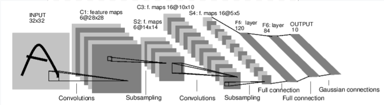
convnet¶

這是一個簡單的前饋網路。它獲取輸入，將其依次通過幾個層，然後最終給出輸出。

神經網路的典型訓練過程如下

定義具有一些可學習參數（或權重）的神經網路
迭代輸入的數據集
通過網路處理輸入
計算損失（輸出與正確答案的差距有多大）
將梯度反向傳播到網路的參數中
更新網路的權重，通常使用一個簡單的更新規則：weight = weight - learning_rate * gradient

定義網路¶

讓我們定義這個網路

import torch
import torch.nn as nn
import torch.nn.functional as F


class Net(nn.Module):

    def __init__(self):
        super(Net, self).__init__()
        # 1 input image channel, 6 output channels, 5x5 square convolution
        # kernel
        self.conv1 = nn.Conv2d(1, 6, 5)
        self.conv2 = nn.Conv2d(6, 16, 5)
        # an affine operation: y = Wx + b
        self.fc1 = nn.Linear(16 * 5 * 5, 120)  # 5*5 from image dimension
        self.fc2 = nn.Linear(120, 84)
        self.fc3 = nn.Linear(84, 10)

    def forward(self, input):
        # Convolution layer C1: 1 input image channel, 6 output channels,
        # 5x5 square convolution, it uses RELU activation function, and
        # outputs a Tensor with size (N, 6, 28, 28), where N is the size of the batch
        c1 = F.relu(self.conv1(input))
        # Subsampling layer S2: 2x2 grid, purely functional,
        # this layer does not have any parameter, and outputs a (N, 6, 14, 14) Tensor
        s2 = F.max_pool2d(c1, (2, 2))
        # Convolution layer C3: 6 input channels, 16 output channels,
        # 5x5 square convolution, it uses RELU activation function, and
        # outputs a (N, 16, 10, 10) Tensor
        c3 = F.relu(self.conv2(s2))
        # Subsampling layer S4: 2x2 grid, purely functional,
        # this layer does not have any parameter, and outputs a (N, 16, 5, 5) Tensor
        s4 = F.max_pool2d(c3, 2)
        # Flatten operation: purely functional, outputs a (N, 400) Tensor
        s4 = torch.flatten(s4, 1)
        # Fully connected layer F5: (N, 400) Tensor input,
        # and outputs a (N, 120) Tensor, it uses RELU activation function
        f5 = F.relu(self.fc1(s4))
        # Fully connected layer F6: (N, 120) Tensor input,
        # and outputs a (N, 84) Tensor, it uses RELU activation function
        f6 = F.relu(self.fc2(f5))
        # Gaussian layer OUTPUT: (N, 84) Tensor input, and
        # outputs a (N, 10) Tensor
        output = self.fc3(f6)
        return output


net = Net()
print(net)

Net(
  (conv1): Conv2d(1, 6, kernel_size=(5, 5), stride=(1, 1))
  (conv2): Conv2d(6, 16, kernel_size=(5, 5), stride=(1, 1))
  (fc1): Linear(in_features=400, out_features=120, bias=True)
  (fc2): Linear(in_features=120, out_features=84, bias=True)
  (fc3): Linear(in_features=84, out_features=10, bias=True)
)

您只需要定義 forward 函數，並且 backward 函數（計算梯度的地方）會使用 autograd 自動為您定義。您可以在 forward 函數中使用任何 Tensor 運算。

模型的學習參數由 net.parameters() 返回

params = list(net.parameters())
print(len(params))
print(params[0].size())  # conv1's .weight

10
torch.Size([6, 1, 5, 5])

讓我們嘗試一個隨機的 32x32 輸入。注意：此網路 (LeNet) 的預期輸入大小為 32x32。要在 MNIST 數據集上使用此網路，請將數據集中的影像調整大小為 32x32。

input = torch.randn(1, 1, 32, 32)
out = net(input)
print(out)

tensor([[ 0.1453, -0.0590, -0.0065,  0.0905,  0.0146, -0.0805, -0.1211, -0.0394,
         -0.0181, -0.0136]], grad_fn=<AddmmBackward0>)

使用隨機梯度將所有參數的梯度緩衝區歸零並進行反向傳播

net.zero_grad()
out.backward(torch.randn(1, 10))

注意

torch.nn 僅支援小批量。整個 torch.nn 套件僅支援作為樣本小批量的輸入，而不是單個樣本。

例如，nn.Conv2d 將接收 nSamples x nChannels x Height x Width 的 4D Tensor。

如果您只有一個樣本，只需使用 input.unsqueeze(0) 添加一個假的批次維度。

在繼續之前，讓我們回顧一下到目前為止您所看到的所有類別。

回顧

torch.Tensor - 一個多維陣列，支援像 backward() 這樣的自動微分運算。也保持著梯度 w.r.t. 張量。
nn.Module - 神經網路模組。封裝參數的便捷方法，帶有將它們移動到 GPU、匯出、加載等的輔助函數。
nn.Parameter - 一種類型的 Tensor，當分配為 Module的屬性時，會自動註冊為參數。
autograd.Function - 實作 *autograd 運算的 forward 和 backward 定義*。每個 Tensor 運算都會建立至少一個 Function 節點，該節點連接到建立 Tensor 的函數，並*編碼其歷史記錄*。

到目前為止，我們已經涵蓋了

定義神經網路
處理輸入並呼叫 backward

還剩下

計算 loss
更新網路的權重

Loss Function¶

Loss function 接受一對 (output, target) 輸入，並計算一個值來估計 output 與 target 之間的差距。

在 nn 套件下有幾種不同的 loss functions。一個簡單的 loss function 是：nn.MSELoss，它計算 output 和 target 之間的均方誤差。

例如

output = net(input)
target = torch.randn(10)  # a dummy target, for example
target = target.view(1, -1)  # make it the same shape as output
criterion = nn.MSELoss()

loss = criterion(output, target)
print(loss)

tensor(1.3619, grad_fn=<MseLossBackward0>)

現在，如果您沿著 backward 方向追蹤 loss，使用其 .grad_fn 屬性，您將看到一個類似於以下的計算圖

input -> conv2d -> relu -> maxpool2d -> conv2d -> relu -> maxpool2d
      -> flatten -> linear -> relu -> linear -> relu -> linear
      -> MSELoss
      -> loss

因此，當我們呼叫 loss.backward() 時，整個圖會針對神經網路參數進行微分，並且圖中所有具有 requires_grad=True 的 Tensors 都會將它們的 .grad Tensor 累加梯度。

為了說明，讓我們向後追蹤幾個步驟

print(loss.grad_fn)  # MSELoss
print(loss.grad_fn.next_functions[0][0])  # Linear
print(loss.grad_fn.next_functions[0][0].next_functions[0][0])  # ReLU

<MseLossBackward0 object at 0x7f428dcaf520>
<AddmmBackward0 object at 0x7f428dcaf580>
<AccumulateGrad object at 0x7f428dcad510>

Backprop¶

要反向傳播誤差，我們只需要執行 loss.backward()。您需要清除現有的梯度，否則梯度將會被累積到現有梯度中。

現在我們將呼叫 loss.backward()，並查看 backward 之前和之後 conv1 的 bias 梯度。

net.zero_grad()     # zeroes the gradient buffers of all parameters

print('conv1.bias.grad before backward')
print(net.conv1.bias.grad)

loss.backward()

print('conv1.bias.grad after backward')
print(net.conv1.bias.grad)

conv1.bias.grad before backward
None
conv1.bias.grad after backward
tensor([ 0.0081, -0.0080, -0.0039,  0.0150,  0.0003, -0.0105])

現在，我們已經了解如何使用 loss functions。

稍後閱讀

神經網路套件包含各種模組和 loss functions，這些模組和 loss functions 構成了深度神經網路的構建模組。完整的清單和文件位於這裡。

唯一剩下要學習的是

更新網路的權重

更新權重¶

實務中最簡單的更新規則是 Stochastic Gradient Descent (SGD)

weight = weight - learning_rate * gradient

我們可以使用簡單的 Python 程式碼來實現這一點

learning_rate = 0.01
for f in net.parameters():
    f.data.sub_(f.grad.data * learning_rate)

但是，當您使用神經網路時，您會想要使用各種不同的更新規則，例如 SGD、Nesterov-SGD、Adam、RMSProp 等。為了實現這一點，我們建立了一個小套件：torch.optim，它實現了所有這些方法。使用它非常簡單

import torch.optim as optim

# create your optimizer
optimizer = optim.SGD(net.parameters(), lr=0.01)

# in your training loop:
optimizer.zero_grad()   # zero the gradient buffers
output = net(input)
loss = criterion(output, target)
loss.backward()
optimizer.step()    # Does the update

注意

請注意如何使用 optimizer.zero_grad() 手動將梯度緩衝區設定為零。這是因為梯度會如 Backprop 節中所述進行累積。

指令碼的總執行時間： ( 0 分鐘 0.036 秒)

由 Sphinx-Gallery 產生圖庫